Pages

Wednesday, April 25, 2018

Simple poll aggregation models

I have played some more with my simplified poll aggregation models using Henderson moving averages (HMA) and Locally Weighted Scatter-plot Smoothing (LOWESS). I fit the smoothed curve taking account of house biases (that is, the systemic tendency for a pollster to favour one house or the other). The models are fit iteratively, with the objective of adjusting the estimated house effects to minimize the sum of the errors squared for the fit. I have also compared these models with the Hierarchical Bayesian model I use.

Cutting to the chase: the plot of the various aggregation models follows. Just under the plot heading you can see the end-point for each of the models (as at 22 April 2018). As usual, the input data for these models comes from the Wikipedia page on the Next Australian Federal Election.


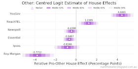
The estimated house biases (the first six columns expressed in pro-Coalition percentage points) for each model (the rows) are in the next table. Note, these are relative house effects as the rows have been constrained to sum to zero. The "Iter" column is the number of iterations taken to produce this estimate. The "Sum Errors Squared" column is the sum of the errors squared, noting that within the model these are calculated from proportions (between 0 and 1) and not percentage points (between 0 and 100).

Essential Ipsos Newspoll ReachTEL Roy Morgan YouGov Iter Sum Errors Squared
Model
HMA-181 -0.845100 -0.568599 -0.615695 -0.408452 0.278507 2.159338 13 0.008061
HMA-365 -0.832409 -0.485705 -0.589923 -0.401716 0.150488 2.159266 12 0.008920
LOWESS-91 -0.818754 -0.554349 -0.604249 -0.403321 0.216127 2.164546 13 0.008110
LOWESS-181 -0.826693 -0.475102 -0.577678 -0.413161 0.169364 2.123270 12 0.009222

This compares well with the Hierarchical Bayesian model:


The updated code follows.
# PYHTON: iterative data fusion: 
#   using Henderson Moving Averages (HMA)
#   and Locally Weighted Scatterplot Smoothing (LOWESS)
#   with a sum-to-zero adjustment for House biases 

import pandas as pd
import numpy as np
from numpy import dot
import matplotlib.pyplot as plt
import matplotlib.dates as mdates
import statsmodels.api as sm
lowess = sm.nonparametric.lowess

import sys
sys.path.append( '../bin' )
from mg_plot import mg_min_max_end
from Henderson import Henderson
plt.style.use('../bin/markgraph.mplstyle')


# --- key constants
HMA_PERIODS = [181, 365] # days
LOWESS_PERIODS = [91, 181] # days
MODALITIES = ['HMA', 'LOWESS']

graph_dir = './Graphs/'
graph_leader = 'FUSION-'
intermediate_data_dir = "./Intermediate/"


# --- Functions
def note_house_effects(effects, Houses, mode, period, 
    iter_count, current_sum):
    ''' For each iteration we record the results. This function compiles
        the results into a single row DataFrame, which will be appended
        to the iteration history DataFrame
        
        effects:    is a column vector of house effects that was applied
        Houses:     is a list of Houses
        mode:       is a mode in 'HMA' or 'LOWESS'
        iter_count: is the iteration count as an integer
        current_sum: is the error squared sum as a float
        returns:    a Pandas DataFrame with one row
    '''
    house_effects = pd.DataFrame([effects.T[0]], 
        columns=Houses, index=[iter_count])
    house_effects['Iterations'] = iter_count
    house_effects['Model'] = '{}-{}'.format(mode, period)
    house_effects['Error Sq Sum'] = [current_sum]
    house_effects['Effects Sq Sum'] = dot(effects.T, effects)[0]
    return house_effects

def interpolate_and_smooth(x):
    ''' interpolate missing data in a series then apply 
        a 21-term moving average - with smaller moving averages 
        at the end of the series.
        
        x:          a Pandas Series
        returns:    a Pandas Series
    '''
    # set up smoothers - note centre weighting in 7- and 21-term MA
    smoother21 = np.array([1,1,2,2,3,3,3,3,3,3,3,3,3,3,3,3,3,2,2,1,1])
    smoother21 = smoother21 / np.sum(smoother21)
    smoother7 = np.array([1,2,3,3,3,2,1]) # 7-term MA
    smoother7 = smoother7 / np.sum(smoother7)
    smoother3 = np.array([1,1,1])
    smoother3 = smoother3 / np.sum(smoother3)
    
    x = x.interpolate()
    
    # calculate smoothers
    s21 = x.rolling(window=len(smoother21), min_periods=len(smoother21), 
        center=True).apply(func=lambda x: (x * smoother21).sum()) 
    s7 = x.rolling(window=len(smoother7), min_periods=len(smoother7), 
        center=True).apply(func=lambda x: (x * smoother7).sum()) 
    s3 = x.rolling(window=len(smoother3), min_periods=len(smoother3), 
        center=True).apply(func=lambda x: (x * smoother3).sum()) 
        
    # fix the end data from smoothed to less smoothed to unsmoothed 
    s = s7.where(s21.isnull(), other=s21) 
    s = s3.where(s.isnull(), other=s) 
    s = x.where(s.isnull(), other=s) 
    
    return(s)

def estimate_hidden_states(ydf, mode, period, n_days):
    ''' This function takes the house-effect adjusted y values and 
        estimates a hidden vote share for each day under analysis using 
        moving averages to give a smooth result.
       
        ydf:        is a DataFram of y values, 
                    with cols: Day and adjusted_y
        mode:       is a MODALITY string - either 'HMA' or 'LOWESS'
        period:     in days - the span for the moving average
        returns:    a pandas Series indexed by days
    '''

    # --- plot known data points and interpolate the in-between days
    #     where more than one poll on a day, average those polls.
    hidden_state = pd.Series(np.array([np.nan] * n_days))
    for day in ydf['Day'].unique():
        result = ydf[ydf['Day'] == day]
        hidden_state[day] = result['adjusted_y'].mean()
    
    # --- apply the HMA or LOWESS smoothing 
    if mode == 'HMA':
        # HMA requires data points for all x values
        # therefore we interpolate first
        hidden_state = interpolate_and_smooth(hidden_state)
        hidden_state = Henderson(hidden_state, period)
    elif mode == 'LOWESS':
        # LOWESS does not require data points for all x values
        hidden_state = pd.Series(
            lowess(hidden_state, hidden_state.index, frac=period/n_days, 
            return_sorted=False))
        hidden_state = interpolate_and_smooth(hidden_state)
    else:
        assert(False)
    return hidden_state

def calculate_house_effects(Houses, ydf, hidden_state):
    ''' For a curve generated by the estimate_hidden_states function, 
        calculate the zero-sum constrained house effects for each pollster
        
        Houses:     is a list of pollsters
        ydf:        is a pandas DataFrame of y values/attributes, 
                    with columns y, Day and Firm
        returns:    a column vector of house effects
    '''
    new_effects = []
    for h in Houses:
        count = 0
        sum = 0
        result = ydf[ydf['Firm'] == h]
        for index, row in result.iterrows():
            sum += hidden_state[row['Day']] - row['y']
            count += 1.0
        new_effects.append(sum / count)
    new_effects = pd.Series(new_effects)
    new_effects = new_effects - new_effects.mean() # sum to zero
    effects = new_effects.values
    effects.shape = len(effects), 1 # it's a column vector
    return effects

def sum_error_squared(hidden_state, ydf):
    ''' For a curve generated by the estimate_hidden_states function, 
        calculate the sum of the errors-squared for the y observations
        
        hidden_state: a pandas Series indexed by days
        ydf:        is a pandas DataFrame of y values/attributes, 
                    with columns Day and adjusted_y
        returns:    a float
    '''
    dayValue = hidden_state[ydf['Day']]
    dayValue.index = ydf.index
    e_row = (dayValue - ydf['adjusted_y']).values # row vector
    return dot(e_row, e_row.T)

def get_minima(history):
    ''' Return the minimum sum of errors-squared from the iteration 
        history DataFrane
        
        history:    pandas DataFrame of all iterations to now
        returns:    minimum value for the sum of errors squared
    '''
    return history['Error Sq Sum'].min()

def get_details(search, history, Houses):
    ''' Find the details in the iteration history DataFrame for 
        a specific search value. The search term is the value of 
        sum errors squared being sought (typically a minimum)
        
        search:     the value of sum errors squared being sought
        history:    pandas DataFrame of all iterations to now
        Houses:     is a list of pollsters
        returns:    (iter_num, effects) - found selected effects in history
    '''
    effects = history[history['Error Sq Sum'] == search][Houses].T.values
    effects.shape = (len(effects), 1) # effects is a column vector
    iter_num = history[history['Error Sq Sum'] == search]['Iterations']
    return (iter_num, effects)

def curve_fit(Houses, H, mode, period, ydf, n_days):
    ''' Iteratively fit curves to the data, then adjust the data to
        better reflect the house effects for each pollster. Stop when
        the changes being made become minimal. 
        
        Houses:     is a list of Houses
        H:          is a House Effects dummy var matrix
        mode:       is a MODALITY string - either 'HMA' or 'LOWESS' - 
                    which reflects the type of curve we will fit
        period:     in days - the span for the moving average
        ydf:        pandas DataFrame of y variables with cols 'y', 'Day' 'Firm'
        n_days:     number of days under analysis
        returns:    (iter_count, history, y)
    '''
    # --- initialisation regardless of mode 
    effects = np.zeros(shape=(len(Houses), 1)) # start at zero
    history = pd.DataFrame()
    previous_sum = np.inf
    y = ydf['y'].values
    y.shape = (len(y), 1) # column vector
    iter_count = 0;
    
    # --- iterative fitting process ...
    #   note: this is only a quick and dirty approximation
    print('--> About to iterate: {}-{}'.format(mode, period))
    while True: 
            
        iter_count += 1

        # --- calculate new hidden states, 
        #     update estimate of house effects 
        #     and calculate error squared
        ydf['adjusted_y'] = y + dot(H, effects) # matrix arithmetic 
        hidden_state = estimate_hidden_states(ydf, mode, period, n_days)
        effects = calculate_house_effects(Houses, ydf, hidden_state)
        current_sum = sum_error_squared(hidden_state, ydf)
        if iter_count > 1:
            minima = get_minima(history)
        else:
            minima = np.inf
        # Note: minima does not include current_sum 

        # --- remember where we have been - puts current_sum into history
        house_effects = note_house_effects(effects, Houses, 
            mode, period, iter_count, current_sum)
        history = history.append(house_effects)
        print('--\n', house_effects)
            
        # --- exit when we are no longer making much difference
        margin = 0.000000000001
        if np.abs(current_sum - minima) < margin or np.abs(
                current_sum - previous_sum) < margin:
            # near enough to a minima
            break
        
        # --- end loop tidy-ups
        previous_sum = current_sum

    # --- exit
    return (iter_count, history, y)

def chart(sdf=None, title=None, y_label=None, annotation='', file_prefix=None):    
    ax = sdf.plot()
    ax.set_title(title)
    ax.set_xlabel('')
    ax.set_ylabel(y_label) 
    ax.xaxis.set_major_formatter(mdates.DateFormatter('%b\n%y'))
    ax.text(0.01, 0.99, annotation,
        ha='left', va='top', fontsize='xx-small', 
        color='#333333', transform = ax.transAxes) 

    fig = ax.figure
    fig.set_size_inches(8, 4)
    fig.tight_layout(pad=1)
    fig.text(0.99, 0.01, 'marktheballot.blogspot.com.au',
        ha='right', va='bottom', fontsize='x-small', 
        fontstyle='italic', color='#999999') 
    fig.savefig(graph_dir+file_prefix+'.png', dpi=125) 
    
    return (fig, ax)

# --- collect the model data
# the XL data file was extracted from the Wikipedia
# page on the next Australian Federal Election
workbook = pd.ExcelFile('./Data/poll-data.xlsx')
df = workbook.parse('Data')

# drop pre-2016 election data
df['MidDate'] = [pd.Period(date, freq='D') for date in df['MidDate']]
df = df[df['MidDate'] > pd.Period('2016-07-04', freq='D')] 

# convert dates to days from start
start = df['MidDate'].min()  # day zero
df['Day'] = df['MidDate'] - start # day number for each poll
n_days = df['Day'].max() + 1

# treat later Newspoll as a seperate series 
# for change to one nation treatment
df['Firm'] = df['Firm'].where((df['MidDate'] < pd.Period('2017-12-01', freq='D')) |
    (df['Firm'] != 'Newspoll'), other='Newspoll2')

df = df.sort_values(by='Day')
df.index = range(len(df)) # reindex, just to be sure


# --- do for a number of different HMAs and LOWESS functions
Adjustments = pd.DataFrame()
Hidden_States = pd.DataFrame()

for mode in MODALITIES:

    if mode == 'HMA':
        PERIODS = HMA_PERIODS
    elif mode == 'LOWESS':
        PERIODS = LOWESS_PERIODS
    else:
        assert(False)

    for period in PERIODS:

        # --- initialisation - in preparation to fit iteratively
        ydf = pd.DataFrame([df['TPP L/NP'] / 100.0, df['Day'], df['Firm']], 
            index=['y', 'Day', 'Firm']).T
        H = pd.get_dummies(df['Firm']) # House Effects dummy var matrix
        Houses = H.columns
        H = H.as_matrix()
        
        # --- undertake the analysis ...
        (iter_count, history, y) = curve_fit(Houses, H, mode, period, ydf, n_days)
        
        # --- record the minima generating house effects 
        minima = get_minima(history)
        (iter_num, effects) = get_details(minima, history, Houses)
        ydf['adjusted_y'] = y + dot(H, effects)
        hidden_state = estimate_hidden_states(ydf, mode, period, n_days)
        print(type(hidden_state.index))
        Hidden_States['{}-{}'.format(mode, period)] = hidden_state
        sum = sum_error_squared(hidden_state, ydf)
        effects = calculate_house_effects(Houses, ydf, hidden_state)
        house_effects = note_house_effects(effects, Houses, 
            mode, period, iter_count, sum)
        Adjustments = Adjustments.append(house_effects)
        
        # get back to something useful
        hidden_state *= 100.0
        hidden_state.index = [(start + x).to_timestamp().date() 
        for x in hidden_state.index]
        
        fax = chart(sdf=hidden_state, 
            title='{}-{}: Coalition TPP Vote Share'.format(mode, period), 
            y_label='Percent Coalition TPP Vote', 
            file_prefix=graph_leader+'{}-{}'.format(mode, period))

        fax = mg_min_max_end(series=hidden_state, fax=fax,
            filename=graph_dir+graph_leader+
            '{}-{} !annotated.png'.format(mode, period))
        plt.close() 
        
        print('\n-- FOUND --\n', house_effects, '\n-----------\n')

# --- get an Adjustments summary in pro-Coalition percentage points
Adjustments.index = Adjustments['Model']
AdjustmentsX = Adjustments[Houses] * -100 # Note: bias = -treatment * 100%
#AdjustmentsX['Total'] = AdjustmentsX.sum(axis=1)
AdjustmentsX['Iter'] = Adjustments['Iterations']
AdjustmentsX['Sum Errors Squared'] = Adjustments['Error Sq Sum']
print(AdjustmentsX.to_html())
print(AdjustmentsX)


# --- Plot
Hidden_States *= 100.0 # from proportions back to percent
Bayes_TPP = pd.read_csv(intermediate_data_dir+
    'STAN-TPP-ZERO-SUM-walk.csv', 
    header=0, index_col=0, quotechar='"', sep=',', 
    na_values = ['na', '-', '.', '']) 
Hidden_States['Bayes'] = Bayes_TPP['median']
Hidden_States.index = [(start + x).to_timestamp().date() 
        for x in Hidden_States.index]

# allow us to annotate the end points
endpoints = Hidden_States[-1:].copy().round(1)
endpoints = 'Endpoints: ' + '; '.join([x+': '+str(y)+'%' 
    for x,y in zip(endpoints.columns, endpoints[0:1].values[0])])

# and plot ...
fig, ax = chart(sdf=Hidden_States, title='Coalition TPP Poll Aggregates [Sum(HE)==0]', 
    y_label='Percent Coalition TPP Vote', annotation=endpoints, 
    file_prefix=graph_leader+'!Comparative')
plt.close() 

combination = ', '.join(Hidden_States.columns.values)
Hidden_States['Average'] = Hidden_States.mean(axis=1)

fax = chart(sdf=Hidden_States['Average'], 
    title='Combined Coalition Aggregate TPP Vote Share', 
    y_label='Percent Coalition TPP Vote', annotation=combination, 
    file_prefix=graph_leader+'!Comparative !combined')

fax = mg_min_max_end(series=Hidden_States['Average'], fax=fax,
    filename=graph_dir+graph_leader+'!Comparative !combined !annotated.png')
plt.close() 

Saturday, April 14, 2018

Betting markets

As we inch towards for the 2019 Australian Federal Election I am now turning my mind to betting markets, and keeping track of the odds book-makers provide on the winner of the election.

Unlike for the 2016 election, bookmakers are typically offering odds on wildly improbable outcomes: that the Prime Minister will come from Pauline Hanson's One Nation, the Greens, or even the Australian Conservatives. Bookmakers include such improbable options to maximise profits. And they include these options at odds that overstate the real probability of the next Prime Minister coming from one of those parties. It is an example of a longshot-bias in betting markets.

There appears to be two drivers for the longshot bias. First, punters seem to systemically over-estimate the probability of a longshot outcome. Second, bookmakers can be risk adverse at the very long end of a market. They are often loath to list odds longer than (say) 100 to 1, because the bookmaker carries the risk that the listing could be costly should the longshot come in with a late bet on the longshot.

As I did with the individual seat odds for the 2016 election, to correct for the longshot bias, I am ignoring the over-inflated odds in respect of the minor parties forming government after the next federal election.

My first automated collection of odds, and the implied Coalition win probabilities follows.

House Coalition Odds ($) Labor Odds ($) Coalition Win Probability (%)
2018-04-14 Ladbrokes 2.50 1.40 35.90
2018-04-14 CrownBet 2.40 1.50 38.46
2018-04-14 Sportsbet 3.00 1.37 31.35

The automated collection of odds requires me to write a web-scraper for each online bookmaker. For some bookmakers this is relatively easy to do. However scraping is more difficult with those bookmakers that use JavaScript to construct their web-pages dynamically. It takes time to write bespoke web-scrapers. My go to tools for web-scraping are Beautiful Soup and Selenium.

Monday, April 9, 2018

The Newspoll 30 Aggregation

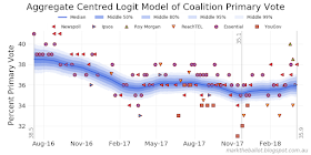
The three most recent polls (Newspoll, Ipsos and Roy Morgan) have all been more benign for Malcolm Turnbull than earlier polls this year. This yields an aggregation that continues to improve (albeit slowly) for the Coalition. Nonetheless, the Labor party remains the strong favourite to win if an election was held at the moment.

In the next few charts we will look at the two-party preferred (TPP) vote share, first through the lens of the Bayesian Hierarchical model, then using Henderson moving averages (HMA) and locally weighted scatter plot smoothing (LOWESS). All of these charts assume that systemic house effects sum to zero.


The next set of charts provides the aggregations for primary vote shares.


Which yields a TPP estimate, using preference flows from previous elections.


Note: this analysis uses data from the Wikipedia page on the next Australian election. Further details on the Bayesian models I use can be found here.

Monday, April 2, 2018

Data Fusion and House Effects

I was wondering whether I could use the (famous) Kalman Filter as a quick cross-check of my house bias calculations in Stan. As I contemplated the problem, a few things occurred to me:
  • The Kalman Filter is designed for multivariate series - I am working with a univariate series - not a problem (and the math is much simpler), but it doesn't take advantage of the power of the Kalman Filter
  • The beauty of the Kalman Filter is that it balances process control information (a mathematical model of what is expected) with measurement or sensor information - where my series is a random walk without any process control information
  • In its simpler forms, it assumes that the period between sensor readings is constant - whereas poll timing is variable, with lengthy gaps over Christmas for example
  • In its simpler forms, it assumes that sensor readings occur concurrently - whereas poll readings from different polling firms rarely appear on the same day, for the same period of analysis
  • And in its simpler forms, the Kalman Filter is not designed for sparse sensor readings - as this results in an overly high covariance from one period to the next when there are no sensor readings - in the current case we have almost 700 days under analysis and around 100 polls from 6 pollsters.

In short, it looked like my hoped-for solution would be too difficult (at least for me) to quickly implement at a level of complexity necessary for my problem. Not all wasted, it became clear to me why the Kalman Filters others have implemented (only using polling days as the unit of analysis) were so noisy. I also realised that my Stan program has a similar issue to the last one listed above: when I use weeks rather than days as the period/unit of analysis, I get a noisier result.

I then wondered if there was another method of data fusion, which would iteratively derive an estimate of the house bias, and which could be assessed against reducing the sum of the error squared (between the smoothed aggregation and the bias-adjusted poll results). I decided to use long-term Henderson moving averages (HMA) for this purpose. [Another possibility was a LOESS or localised regression].

Before we get to that let's quickly recap the the current estimate of two-party preferred (TPP) vote share and more importantly for this exercise, the house effects. It is important to note that the house effects here are constrained to sum to zero. We have maintained that constraint in the HMA work.


The full set of April 2018 updated poll aggregates can be found here.

For the analysis, I looked at four different HMAs: 91, 181, 271 and 365 days, which is roughly 3, 6, 9 and 12 months. The resulting best fit curves for each case follows. But please note, in these charts I have not plotted the original poll results, but the bias-adjusted poll results. For example, if you look at YouGov in the above chart there are a cluster of YouGov polls at 50 per cent from July to December 2017. In the charts below, these polls have been adjusted downwards by about two and a quarter percentage points.


We can compare these results with the original Bayesian analysis as follows. Of note, the Bayesian estimate I calculate in Stan is less noisy that any of the HMAs above. Of some comfort, there is a strong sense that these lines are similar, albeit with more or less noise.


So we get to the crux of things, how does the house bias estimated in the Bayesian process by Stan compare with the quick and dirty analyses above? The following table gives the results, including the number of iterations it took to find the line of best (or at least reasonably good) fit.

Essential Ipsos Newspoll ReachTEL Roy Morgan YouGov Iterations
HMA-91 -0.737809 -0.730556 -0.632002 -0.233041 0.020941 2.312468 32
HMA-181 -0.756775 -0.674001 -0.611148 -0.297269 0.106231 2.232961 4
HMA-271 -0.715895 -0.538550 -0.557863 -0.295559 -0.145591 2.253458 3
HMA-365 -0.728708 -0.535313 -0.562754 -0.292410 -0.122263 2.241449 3
Bayesian Est -0.7265 -0.6656 -0.5904 -0.2619 0.1577 2.1045 --

The short answer is that our results are bloody close! Not too shabby at all!

For those interested in this kind of thing, the core python code follows (minus the laborious plotting code). It is a bit messy, I have used linear algebra for some of the calculations, and others I have done in good-old-fashioned for-loops. If I wanted to be neater, I should have used linear algebra through-out. Next time I promise.

# PYHTON: iterative data fusion 
#           using Henderson moving averages

import pandas as pd
import numpy as np
from numpy import dot
import matplotlib.pyplot as plt
import matplotlib.dates as mdates

import sys
sys.path.append( '../bin' )
from Henderson import Henderson
from mg_plot import *
plt.style.use('../bin/markgraph.mplstyle')

# --- key constants
HMA_PERIODS = [91, 181, 271, 365] # 3, 6, 9, 12 months
graph_dir = './Graphs-HMA/'
graph_leader = 'HMA-'
intermediate_data_dir = "./Intermediate/"

# --- collect the model data
# the XL data file was extracted from the Wikipedia
# page on next Australian Federal Election
workbook = pd.ExcelFile('./Data/poll-data.xlsx')
df = workbook.parse('Data')

# drop pre-2016 election data
df['MidDate'] = [pd.Period(date, freq='D') for date in df['MidDate']]
df = df[df['MidDate'] > pd.Period('2016-07-04', freq='D')] 

# convert dates to days from start
start = df['MidDate'].min()  # day zero
df['Day'] = df['MidDate'] - start # day number for each poll
n_days = df['Day'].max() + 1

df = df.sort_values(by='Day')
df.index = range(len(df)) # reindex, just to be sure

# --- do for a number of different HMAs
Adjustments = pd.DataFrame()
Hidden_States = pd.DataFrame()
for HMA_PERIOD in HMA_PERIODS:

    # --- iniialisation
    y = (df['TPP L/NP'] / 100.0).as_matrix()
    ydf = pd.DataFrame([y, df['Day'], df['Firm']], 
        index=['y', 'Day', 'Firm']).T
    y.shape = len(y), 1 # a column vector
    H = pd.get_dummies(df['Firm']) # House Effects dummy matrix
    Houses = H.columns
    effects = np.zeros(len(H.columns))
    effects.shape = len(H.columns), 1 # a column vector
    H = H.as_matrix()

    # --- iteration
    current_sum = np.inf
    iteration_count = 0
    effects = np.zeros(len(Houses))
    effects.shape = len(Houses), 1 # column vector
    hidden_state = pd.Series(np.array([np.nan] * n_days))
    while True: 

        # --- save best for later
        ydf_old = ydf.copy()
        hidden_state_old = hidden_state.copy()
        house_effects = pd.DataFrame([(-100 * effects.T)[0]], 
            columns=Houses, index=[['HMA-{}'.format(HMA_PERIOD)]])
        house_effects['Iterations'] = [iteration_count]
    
        # --- estimate the hidden state
        ydf['adjusted_y'] = y + dot(H, effects)
        hidden_state = pd.Series(np.array([np.nan] * n_days))
        for day in ydf['Day'].unique():
            result = ydf[ydf['Day'] == day]
            hidden_state[day] = result['adjusted_y'].mean()
        hidden_state = hidden_state.interpolate()
        hidden_state = Henderson(hidden_state, HMA_PERIOD)
    
        # --- update the assessment of House Effects
        new_effects = []
        for h in Houses:
            count = 0
            sum = 0
            result = ydf[ydf['Firm'] == h]
            for index, row in result.iterrows():
                sum += hidden_state[row['Day']] - row['y']
                count += 1.0
            new_effects.append(sum / count)
        new_effects = pd.Series(new_effects)
        new_effects = new_effects - new_effects.mean() # sum to zero
        effects = new_effects.values
        effects.shape = len(effects), 1 # it's a column vector

        # --- calculate the sum error squared for this iteration
        previous_sum = current_sum
        dayValue = hidden_state[ydf['Day']]
        dayValue.index = ydf.index
        e_row = (dayValue - ydf['adjusted_y']).values # row vector
        e_col = e_row.copy()
        e_col.shape = len(e_col), 1 # make a column vector
        current_sum = dot(e_row, e_col)[0]

        # exit if not improving solution
        if (current_sum >= previous_sum):
            break
        iteration_count += 1

    # --- get best fit - ie the previous one
    ydf = ydf_old
    hidden_state = hidden_state_old
   
    # --- record house effects 
    Adjustments = Adjustments.append(house_effects)
    Hidden_States['HMA-{}'.format(HMA_PERIOD)] = hidden_state

My Henderson Moving Average python code is here.

Update 6pm 2 April 2018

Having noted above that I could have used a localised regression rather than a Henderson moving average, I decided to have a look.


And the house bias estimates ... again looking good ...

Essential Ipsos Newspoll ReachTEL Roy Morgan YouGov Iterations
LOWESS-61 -0.736584 -0.713434 -0.592154 -0.235112 -0.029474 2.306759 3
LOWESS-91 -0.751777 -0.676071 -0.603489 -0.285200 0.082462 2.234075 17
LOWESS-181 -0.722463 -0.548346 -0.552024 -0.288691 -0.128377 2.239902 3
LOWESS-271 -0.751364 -0.566553 -0.566039 -0.288767 -0.059591 2.232314 2
Bayesian Est -0.7265 -0.6656 -0.5904 -0.2619 0.1577 2.1045 --

Bringing it all together in one chart ...


Which can be averaged as follows: