I have been busy coding a new primary vote aggregation model in Stan and Python. It was an interesting experience as I came to terms with the way in which Stan differs from JAGS (and the ways in which the Hamiltonian Monte Carlo sampling differs from Gibbs sampling). While I found Stan a little more fiddly to code, it is definitely easier to debug, requires fewer iterations, and is therefore faster to both code and run. I will write a technical post shortly on the primary vote aggregation model, as well as some of my experiences with Stan.
So let's get down to the data. First, however, an acknowledgement: I sourced the polling data from the Wikipedia page on the next Australian federal election.
The two-party preferred (TPP) aggregation tends to significant levels of smoothing. At the start of March this model estimates the Coalition would win 47.3 per cent of the TPP vote share. While I have not converted this to an election outcome probability (the next task), this result is strongly suggestive of sizable Labor win, were an election held at the moment.
Next we will look at the primary vote aggregation model I have just completed. This model is not as smoothed as the TPP aggregation model. It is more sensitive to week-on-week polling changes. It is an interesting question whether this is just picking up noise or better listening to the underlying signal.
Of note is the recent decline in primary vote share for Labor and the
Coalition. These votes have moved to the Greens and the other parties.
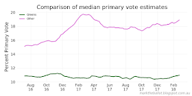
The above charts can be summarised and compared as follows:
The house adjustments are more complicated than for the TPP model. The sum to zero constraint needs to be maintained in two directions simultaneously: for each pollster across the four party groups; and for each party, across the (currently) five pollsters in the data. It is this two-way necessity that sees the median lines sometime appear to sit above or below the preponderance of polling results.
For the primary vote estimates we can calculate a TPP estimate using the preference flows evidenced at the previous election. In this model, I attribute the Other vote share in a single transfer. I do this using the preference flows from the previous elections. Pollsters can be more nuanced because they capture the specific other party from their respondents. They can then apply the actual previous election preference transfer rate for the specific primary party vote nominated by the respondent. [Another acknowledgement: I used Antony Green's reporting on preference flows].
Of note: when the polls are suggesting almost 30 per cent of the primary vote is not going to the major Coalition and Labor parties, how preferences flow will substantially shape the final election outcome. There is a 1.7 percentage point difference in the final TPP estimate between the application of the 2010 and 2016 preference flows.
This can be summarised as follows.


No comments:
Post a Comment