Clearly, circumstances require me to make a similar adjustment to my Bayesian aggregations.
I have used the snap Morgan poll to test my updated aggregation with the Gillard-Rudd discontinuity. This is only a test, as the latest Morgan poll is an SMS poll (not the multi-mode series the Bayesian aggregation expects). I will back-out this SMS data from the model when further polling data becomes available.
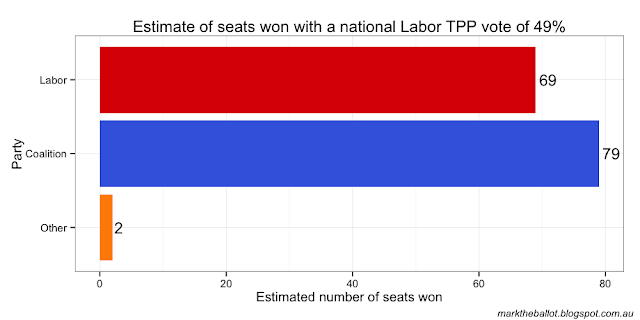
Anyway, I thought it would be interesting to provide the charts from this test, as well as the JAGS code I am using. It certainly suggests a much more competitive election contest. With all the caveats of data inconsistencies, and only having the results from one poll, our very early estimate of the Rudd Resurrection effect is 4.7 percentage points.
    model {
        ## Based on Simon Jackman's model, with an additional element for
        ## the various rounding effects of the different polling houses
        ## and a sum-to-zero constraint on house effects
        ## Update: also provides for a discontinuity with the Gillard to Rudd transition.

        ## -- observational model
        for(poll in 1:NUMPOLLS) { # for each poll result
            roundingEffect[poll] ~ dunif(-houseRounding[poll], houseRounding[poll])
            yhat[poll] <- houseEffect[house[poll]] + walk[day[poll]] +
                roundingEffect[poll]
            y[poll] ~ dnorm(yhat[poll], samplePrecision[poll]) # distribution
        }

        ## -- temporal model
        for(i in 2:PERIOD) { # for each day under analysis ...
            dayToDayAdjust[i] <- ifelse(i==DISCOUNTINUITYDAY, walk[i-1]+discontinuityValue, walk[i-1])
            walk[i] ~ dnorm(dayToDayAdjust[i], walkPrecision)
        }

        ## -- sum-to-zero constraint on house effects (ignoring Morgan F2F)
        #houseEffect[1] <- -sum( houseEffect[2:HOUSECOUNT] ) + houseEffect[MORGANF2F]
        houseEffect[1] <- -sum( houseEffect[2:HOUSECOUNT] )

        ## -- priors
        sigmaWalk ~ dunif(0, 0.0025)        ## uniform prior on std. dev.
        walkPrecision <- pow(sigmaWalk, -2) ##   for the day-to-day random walk
        walk[1] ~ dunif(0.0, 1.0)           ## initialisation of the daily walk
        discontinuityValue ~ dunif(-0.15, 0.15) ## uninformative prior

        for(i in 2:HOUSECOUNT) { ## vague normal priors for house effects
            houseEffect[i] ~ dnorm(0, pow(0.1, -2))
        }
    }


No comments:
Post a Comment