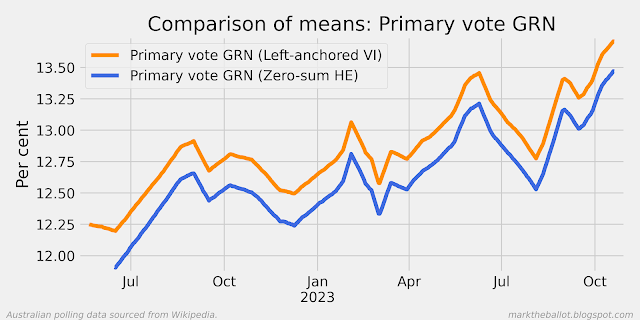
Showing posts with label wonkish. Show all posts

Friday, April 26, 2024

Has Resolve Strategic changed its polling methodology?

The aggregation models I use make many simplifying assumptions. One assumption is that the polling methodology adopted by each polling firm remains unchanged over time. If a pollster indicates that they have changed their polling methodology, then I would treat the subsequent polls as a different series to the prior polls. I have done this with Essential when they published a change to their polling methodology.

When I look at the recent polls from Resolve Strategic, it looks like the polls from 2024 are less favourable to Labour than the polls from the prior two years. In the first chart below, we can see that the last poll result was almost four percentage points more favourable to the Coalition than the long term average for Resolve Strategic. In the second chart below, we can see that historically Resolve Strategic has been the most favourable poll for Labor (on average). And in the third chart below, we can see that the individual Resolve Strategic polls in 2022 and 2023 (indicated with the letter h) were often (but not always) well above the aggregation, and two of the three polls in 2024 are not. 


Now, this could be just the usual random noise and chance that comes with statistics. And in coming months we will see a return of the prior patterns of systemic house bias at Resolve Strategic. But this apparent change could also be the result of a change in polling methodology at Resolve Strategic. At the moment I don't know which explanation is the most plausible. While I have looked, I have not seen a statement on any methodology change from Resolve Strategic (please provide a link below in the comments if I have simply missed it).

If this apparent change in house bias is sustained in the next couple of Resolve Strategic polls, I will assume that there has been something of a change in polling methodology, and I will separate the 2024 and subsequent polls into their own series. 

Please note: this is not a criticism of Resolve Strategic. I have enormous respect for all pollsters, and I appreciate that opinion polling is much harder today than it was (say) 35 years ago (when almost every house had a landline and no-one had mobile phones). At the moment, I am just observing that the last three polls from Resolve Strategic perhaps look a little different from the earlier polls, and I am musing why this might be the case. Nonetheless, I would be somewhat disappointed if it turns out that Resolve Strategic has changed its polling methodology but has not communicated how it has changed and why it has changed.

Sunday, November 5, 2023

A Gaussian process latent variable model for smoothing opinion polls

There are two main reasons I have been using Bayesian methods for polling analysis. First, smoothing, so that I can discern the voting intention signal through the fog of noisy and sometimes contradictory opinion polling. Second, I use these methods to detect “house effects”, the tendency of pollsters to systemically (and I assume unintentionally) to favour one political party or the other.

My primary model was built around the notion of a Gaussian Random Walk. This model imagines a hidden daily walk of population voting intention, which only changes a very small amount from day to day. This voting intention is captured imperfectly by opinion polls from time-to-time. The outputs of this model are familiar. We can see the most likely estimate of the population voting intention, as well as the house effects of each pollster. We can either anchor the model to the actual vote at the last election or assume that pollsters are collectively unbiased (ie. collectively the house effects sum to zero).


A quick aside: You will notice in the above voting-intention charts that I have plotted in the background a random selection of 100 of the 10,000 gaussian random walks I drew on in the Bayesian analysis process.

More recently, I have noticed that a few data scientists are using Gaussian Processes to smooth noisy time series data. So, I thought I would give it a go. 

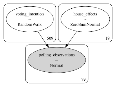
A Gaussian Process approach assumes that the data-points that are taken closer together should be more similar than the data-points that are further apart in time. This is expressed in the model using a function (called a kernel) that quantifies how similar data-points that are closer together should be, and a square covariance matrix that captures the degree of similarity between all the data-points one to another using this function. Rather than model voting intention on every day, this approach only models voting intention on polling days. The kernel function I have used is the Exponentiated Quadratic kernel. Diagrammatically, the model is as follows. 


Priors for the model affect how much smoothing will be applied. With a length_scale around 20, the model produces output that is quite like the Gaussian Random Walk above. 

I am a little intrigued by the small differences between these last two charts and the first two charts above. Because these are still under development, it is entirely possible that I have made an error somewhere. Nonetheless, a possible explanation for some of the small differences might be the tendency for the GP with certain kernels to revert to the mean. This might explain the slightly higher overall level, and the up-tick at the right end of the series. The GRW does not have a mean-reversion bias. 

For the moment, I  will prefer the results of the GRW over the new GP approach. However, I will continue to test, develop, and explore the GP model. 

The primary vote charts follow for completeness.


For those who are particularly interested, the core code for the model follows. For the complete code, you can check out my GitHub site.

def house_effects_model(inputs: dict[str, Any], model: pm.Model) -> pt.TensorVariable:
    """The house effects model."""

    with model:
        house_effect_sigma = 5.0
        house_effects = pm.ZeroSumNormal(
            "house_effects", sigma=house_effect_sigma, shape=inputs["n_firms"]
        )
    return house_effects


def gp_prior(
    inputs: dict[str, Any], 
    model: pm.Model,
    length_scale: Optional[float] = None,
    eta: Optional[float] = None,
) -> pt.TensorVariable:
    """Construct the Gaussian Process (GP) latent variable model prior.
    The prior reflects voting intention on specific polling days.
    
    Note: Reasonably smooth looking plots only emerge with a lenjth_scale
    greater than (say) 15. Divergences occur when eta resolves as being
    close to zero, (which is obvious when you think about it, but also 
    harder to avoid with series that are fairly flat). To address
    these sampling issues, we give the gamma distribution a higher alpha,
    as the mean of the gamma distribution is a/b. And we truncate eta to
    well avoid zero (noting eta is squared before being multiplied by the
    covariance matrix).
    
    Also note: for quick test runs, length_scale and eta can be fixed
    to (say) 20 and 1 respectively. With both specified, the model runs
    in around 1.4 seconds. With one or both unspecified, it takes about 
    7 minutes per run."""

    with model:
        if length_scale is None:
            gamma_hint = {"alpha": 20, "beta": 1}  # ideally a=20, b=1
            length_scale = pm.Gamma("length_scale", **gamma_hint)
        if eta is None:
            eta = pm.TruncatedNormal("eta", mu=1, sigma=5, lower=0.5, upper=20)
        cov = eta**2 * pm.gp.cov.ExpQuad(1, length_scale)
        gp = pm.gp.Latent(cov_func=cov)
        gauss_prior = gp.prior("gauss_prior", X=inputs["poll_day_c_"])
    return gauss_prior


def gp_likelihood(
    inputs: dict[str, Any],
    model: pm.Model,
    gauss_prior: pt.TensorVariable,
    house_effects: pt.TensorVariable,
) -> None:
    """Observational model (likelihood) - Gaussian Process model."""

    with model:
        # Normal observational model
        pm.Normal(
            "observed_polls",
            mu=gauss_prior + house_effects[inputs["poll_firm"]],
            sigma=inputs["measurement_error_sd"],
            observed=inputs["zero_centered_y"],
        )


def gp_model(inputs: dict[str, Any], **kwargs) -> pm.Model:
    """PyMC model for pooling/aggregating voter opinion polls,
    using a Gaussian Process (GP). Note: kwargs allows one to pass
    length_scale and eta to gp_prior()."""

    model = pm.Model()
    gauss_prior = gp_prior(inputs, model, **kwargs)
    house_effects = house_effects_model(inputs, model)
    gp_likelihood(inputs, model, gauss_prior, house_effects)
    return model

Further reading:

Monday, October 30, 2023

Are the polls biased?

I have coded Bayesian aggregations of the polls for the 2025 Federal election.  A key assumption in that aggregation model is that the polls are on average unbiased. While an individual pollsters may have a house effect, collectively I have assumed these house effects sum to zero. 

Another way of looking at the polls is to anchor the model for daily voting intention to the result at the previous election. Under this approach, I assume that there is a collective polling error, and the model allows us to determine the size of that polling error. The model is as follows:


The results for the two party preferred ALP voting intention are as follows.


We can see that on average, if we anchor our model of day-to-day voting intention to the result on election day in May 2022, that our estimate is 1.3 percentage points less favourable to Labor. However, while the polls appear to have a pro-Labor bias, we need to be cautious. Partly because the model is less constrained than the previous model, and partly because there are few polls on the left hand side, the confidence intervals associated with the model are wider than for our zero-sum house effects model. In particular, the model results suggest that the systemic poll error might be anywhere between -1.0 and +3.5 percentage points in Labour's favour. Therefore, while it is more likely than not that the two-party preferred (2pp) polls favour Labor, with these results we cannot be certain. 

The only series where the model is certain that the polls collectively are biased is in respect of Labor's primary vote shares, where the polls appear to be 2.7 percentage points collectively more favourable to Labor. We can be confident as the associated probability density chart below does not have zero within the highest density interval (HDI). While we cannot be certain, it does look like it is more likely than not that some bias is also evident with the Coalition and Other parties primary vote share. 


Friday, October 20, 2023

Voice Referendum 2023

Updated on 25 October and 2 November 2023:

Going into the the Voice Referendum, collectively the polls suggested that the referendum would be lost. There was not one poll predicting a win in the last couple of months before the referendum. This was a win for polling.

Using a Bayesian technique, we can pool the polls. The technique assumes that the voting intention on one day is much like the day before. We can only know the actual voting intention on referendum day. Prior to the referendum, the model assumes the voting intention broadly tracks the opinion polling. The model also assumes that each pollster has an inherent bias. This bias is referred to as an house effect. This is not to suggest that any pollster is deliberately biased. Rather, the bias comes about from systemic factors such as how individual pollsters select and interview their sample, how results are weighted, and so on. However, collectively, this model assumes these biases cancel out (they sum to zero). 

The pooled polls (assuming that individual pollster bias cancelled out) predicted the yes vote would be around 43.4 per cent immediately before the referendum.


As it turned out, this was optimistic. It is now a few weeks since the Voice Referendum was lost. While the count is still progressing, this afternoon (2 Nov) it stood at 39.94% for Yes and 60.06% for No. It is likely that the final count will not differ substantially from this result. 

If we run a similar Bayesian model with the only difference being that this model is pegged to the final referendum result, we can calculate the systemic polling error across all pollsters both individually and collectively.


From the house effects chart immediately above, we can see that (over the entire period under analysis) many pollsters had zero bias within their 95% HDI on average. Nonetheless, some pollsters appear to have over-estimated the yes vote by up to 15 percentage points on average, or underestimated it by around 7 percentage points. 

This was particularly evident with the polling in the first few months of the new Labor government. It is possible that these early polls gave the government false confidence in respect of the winnability of the referendum, and they may have influenced the strategies and tactics adopted by the government towards the referendum. 

Collectively, the modelling suggests that all pollsters were on average 3.4 percentage points too favourable to the level of yes voting intention over the period under analysis. 

Of course, these results are model based, and include a number of modelling assumptions. Care should be taken when interpreting the results. 

The notebook for this analysis can be found here. The data for the analysis came from Wikipedia.

For another perspective see Kevin Boneham.

F

Saturday, April 30, 2022

Are the polls biased?

When you look at the two-party preferred (2pp) election outcome compared with the cloud of 2pp polls immediately prior to an election, it looks like the election result, more often than not, is more favorable to the Coalition than the preceding polls. To put it another way, it looks like the polls on average favour Labor. In the following chart, the election result (in the red/orange box), is typically above most of the polls (blue dots) in the five weeks immediately prior to an election.

If we look specifically at the average of all the 2pp polls in the 14 Federal elections from 1983 (the modern polling era), the Coalition outperformed the final two-week poll average 12 times. Labor outperformed this poll average twice. The following table has the difference between the average 2pp poll for the two weeks prior to the election, and the final 2pp Election result. A negative number indicates the final fortnight polls were on average more favourable to Labor than the election result. A positive number indicates that the polls were more favourable to the Coalition than the election result.

Election Year
Ave Poll Error (for polls concluded in the final 2 weeks before the election)
1983-1.300000
1984-3.400000
1987-2.316667
1990-1.466667
19931.618182
1996-1.941667
1998-0.087500
20010.100000
2004-0.877778
2007-1.500000
2010-2.192308
2013-0.455556
2016-0.327273
2019-3.270000

We can visualise this tendency to favour Labor in the polls as a probability density function, where the area under the curve sums to one. The statistical technique to construct this curve is known as a Kernel Density Estimate (KDE). It is clear, that on average, these polls collectively were a little over one percentage point favourable to Labor when compared with the final Election result.

The next long series of charts shows each of the elections and the way in which the rows in the above table were constructed. Feel free to skip past these charts if this is not your thing.


I have been thinking about whether I can model this bias, and whether I should model it. Using Bayesian techniques, I have found a Student's t-distribution that provides a good algebraic approximation of the probability density function above. So it can be modeled easily. For the nerdy, this distribution has a location of -1.255 percentage points (this is the historic pro-Labor bias), a scale factor of 1.44 percentage points, and 11.22 degrees of freedom.

I am more conflicted on whether I should model the pro-Labor bias. I have not found a compelling theory of action for how the historic bias arose. I assume that the pollsters would rather get the final election result correct (as this reflects well on their business), than to favour one side of politics or the other. It has also been reported to me that this bias does not exist in state government polling. I think this historical bias is unlikely to have occurred by chance alone. Nonetheless, if I don't know why it has occurred in the past, I cannot be confident that the driving factors will persist into the future.

I will think about this some more. If you have any compelling explanations for the historical bias, let me know in the comments below.

Finally, I want to thank Ethan and Rebecca at armariuminterreta.com who compiled this data. Ethan tells me that he in turn was assisted by William Bowe and Kevin Bonham.