Showing posts with label methodology. Show all posts

Wednesday, November 9, 2016

Another polling fail

We have had a few polling fails recently in the Anglo-sphere. Two United Kingdom examples quickly come to mind: the General Election in 2015, where the polls predicted a hung parliament, and Brexit in 2016, in which remaining in the EU was the predicted winner. Closer to home we had the Queensland state election in 2015, in which the polls foreshadowed a narrow Liberal National Party win.

Today's election of Donald Trump in the United States will be added to the list of historic polling fails.

  • The New York Times had the average of the polls with Clinton on 45.9 per cent to Trump's 42.8 per cent (+3.1 percentage points).  The NYT gave Clinton an 84 per cent chance of winning the Electoral College vote.
  • FiveThirtyEight.com had the average of the polls with Clinton on 48.5 to Trump's 44.9 per cent (+3.6). FiveThirtyEight gave Clinton a 71.4 per cent chance of winning the Electoral College vote.
  • The Princeton Election Consortium had Clinton ahead of Trump with +4.0 ± 0.6 percentage points. PEC gave Clinton a 93 per cent chance of winning the Electoral College vote.

While the count is not over, the current tally has Clinton ahead in the national popular vote by +1.1 percentage points, but losing the Electoral College vote. The most likely Electoral College tally looks like Trump with 305 Electoral College votes to Clinton's 233.

So today's big question: Why such a massive polling fail?

It will take some time to answer this question with certainty. However, I have a couple of guesses.

My first guess would be the social desirability bias. This is sometimes referred to as the "shy voter problem" or the Bradley effect. At the core of this polling problem, some voters will not admit their actual polling preference to the pollster because they fear the pollster will negatively judge that preference. It is not surprising that such a controversial figure as Donald Trump would prompt issues of social desirability in polling. Elite opinion was against Trump. Clinton labeled Trump supporters as "deplorable". No-one wants to be in that basket. Pollsters might also look at Latino voters in Florida that appear to have voted for Trump in larger numbers than expected.

The second area where I suspect pollsters will look is their voter turn-out models. Who actually voted compared with who said they would vote to pollsters. This was a very different election to the previous two Presidential elections. Turnout-out models based on previous elections may have misdirected the polling results (particularly on the basis of race and particularly in the industrial mid-west).

A final thing that might be worth looking at is herding. The final polls were close, perhaps remarkably close. This may have been natural, or it may have resulted from pollsters modulating their final outputs to be similar with each other.

Wednesday, July 31, 2013

Further explorations in non-linearity

On the weekend I began exploring a non-linear model for aggregating polling. My test case produced nice looking graphs; but the results were in some large part an artifact of the priors I had chosen for the model (not good).

In the comments to that post, I suggested that part of the problem may have been how I had defined the model.

Thinking about this some more, I think the problem was in this statement: << beta-for-pollster * (poll-result - minimum-poll-result) >>. Rather than the minimum, it should be a central tendency of some type (mid-point, mean, median, etc.).

I have now redefined the model to use the midpoint for each polling house (defined as the (min+max)/2 for that house). The use of house-specific mid-points acknowledges that the raw x scores include the alpha house effect I am trying to estimate. The revised model is:

house-effect-for-pollster = alpha-for-pollster + beta-for-pollster * (poll-result - pollster-mid-point)

The priors to the beta effect have been completely freed-up, so that they are uninformative. As a result, this model works better internally than the previous model.

However, I have added a constraint such that the aggregation assumes the "fizziness" factors also sum to zero. This may be a bollocks assumption; and will need some further analysis.

So - with the caveat that this is still very early exploratory analysis - the results of this new model follow.


On a plain reading, the above charts suggest that the current Rudd effect may actually be better for Labor than other aggregations have found. However, I am not convinced this is anything more than an artifact of the model. I am particularly concerned about the inclusion of data from polling houses that do not have data points across the highs and lows of the Gillard period, and across the Rudd and Gillard periods. Such data don't fully occupy the model, which can result in artifacts.

If we limit the analysis to data from Nielsen and Newspoll for a comparison using data that does fully occupy the model, we get the following.


Because I am committed to presenting poll analysis in a transparent and unbiased fashion, the next two code snippets show how I package up the data for the model (in R), and the model itself (in JAGS).

    # - prepare the data ...
    data$y <- data[ , y] / 100 # vote share between 0-1
    data$variance <- data$y * (1 - data$y) / data$Sample #pq/n
    data$standardError <- sqrt(data$variance)
    data$samplePrecision <- 1 / data$variance
    HOUSES <- levels(data$House)
    HOUSECOUNT <- length(levels(data$House))
    NUMPOLLS <- length(data$y)
    cat('Number of polls: '); print(NUMPOLLS)
    midpoints <- rep(NA, HOUSECOUNT)
    for(i in seq_len(HOUSECOUNT)) {
     midpoints[i] <- (max(data[data$House==HOUSES[i], 'y']) + 
      min(data[data$House==HOUSES[i], 'y'])) / 2
     cat('Midpoints: '); cat(i); cat(' '); cat(HOUSES[i]); cat(': '); print(midpoints[i])
    }
    
    # - remember these dots 
    dotsFile <- paste('./files/', fPrefix, 'original.csv', sep='')
    write.csv(data, file=dotsFile)

    # - manage dates
    day0 <- min(data$Date) - 1  # walk starts from earliest date
    if(endDate == TODAY)
        endDate <- max(data$Date)
    PERIOD <- as.numeric(endDate - day0) # length of walk in days
    DISCOUNTINUITYDAY <- as.numeric(as.Date(discontinuity) - day0)
    cat('Discontinuity: '); print(DISCOUNTINUITYDAY)
    tPrefix <- paste(format(day0+1, '%d-%b-%Y'), ' to ', format(endDate, '%d-%b-%Y'), sep='')
    data$day <- as.numeric(data$Date - day0)

    # - do the MCMC thing ...
    
    parameters <- list(PERIOD = PERIOD,
        HOUSECOUNT = HOUSECOUNT,
        NUMPOLLS = NUMPOLLS,
        DISCOUNTINUITYDAY = DISCOUNTINUITYDAY, 
        NEWSPOLL = which(levels(data$House) == 'Newspoll'),
        y = data$y,
        x = data$y,
        day = data$day,        house = as.integer(data$House),
        samplePrecision = data$samplePrecision,
        midpoints=midpoints
    )
                
    jags <- jags.model(textConnection(model),
        data=parameters,
        n.chains=4,
        n.adapt=n.adapt
    )

    # - burn in
    update(jags, n.iter=n.update) # burn-in the chains

    # - capture results
    jags.capture <- c('walk', 'alpha', 'beta', 'discontinuityValue')
    coda.samples <- coda.samples(jags, jags.capture, n.iter=n.iter, thin=n.thin)
    coda.matrix <- as.matrix(coda.samples)

model {
    ## Derived from Simon Jackman's original model 
    
    ## -- observational model
    for(poll in 1:NUMPOLLS) { 
        # note: x and y are the original polling series
        houseEffect[poll] <- alpha[house[poll]] + 
         beta[house[poll]]*(x[poll]-midpoints[house[poll]]) 
        mu[poll] <- walk[day[poll]] + houseEffect[poll]
        y[poll] ~ dnorm(mu[poll], samplePrecision[poll]) 
    }
            
    ## -- temporal model
    for(i in 2:PERIOD) { # for each day under analysis ...
        day2DayAdj[i] <- ifelse(i==DISCOUNTINUITYDAY, 
            walk[i-1]+discontinuityValue, walk[i-1])
        walk[i] ~ dnorm(day2DayAdj[i], walkPrecision)
    }
    sigmaWalk ~ dunif(0, 0.01)            ## uniform prior on std. dev.  
    walkPrecision <- pow(sigmaWalk, -2)   ##   for the day-to-day random walk
    walk[1] ~ dunif(0.4, 0.6)             ## uninformative prior
    discontinuityValue ~ dunif(-0.2, 0.2) ## uninformative prior

    ## -- house effects model
    for(i in 2:HOUSECOUNT) { ## vague normal priors for house effects
        alpha[i] ~ dunif(-0.1,0.1)
        beta[i] ~ dunif(-1,1) 
    }
    alpha[NEWSPOLL] <- -sum(alpha[2:HOUSECOUNT]) ## sum to zero
    beta[NEWSPOLL] <- -sum(beta[2:HOUSECOUNT]) ## sum to zero
}

Saturday, July 27, 2013

How much was Kevin Rudd worth?

I was a little surprised when I saw Simon Jackman suggest that Kevin Rudd had moved the two-party preferred voting intention by seven percentage points in Labor's favour. It was not consistent with my own analysis and only one pollster (Morgan) has data that supports a seven point movement. Data from all the remaining pollsters suggest the "Rudd Effect" was less than seven percentage points.

Now don't get me wrong, I have enormous respect for Professor Jackman. I purchased and read his 600 page text, Bayesian Analysis for Social Sciences. It is a tour de force on Bayesian statistics. I cannot recommend this book enough. His understanding and knowledge in this area far surpasses my own. Unashamedly, I have used Jackman's approach as the basis for my own aggregation efforts.

However, I suspect he has not noticed that the data since the second ascension of Keven Rudd violates a number of the linear assumptions implicit in his model. In particular, some of the house effects before and after Kevin are radically different. I blogged on this under the rubric: When models fail us. As I noted previously, the violation of the underpinning assumptions results in the model producing incorrect results.

Revisiting the discontinuity model I initially used following Rudd's restoration, I have treated the Morgan, Galaxy and Essential data before and after the restoration as different series. I have also centred the aggregation on the assumption that the house effects for Newspoll and Nielsen sum to zero (this may turn out to be problematic, but it is sufficient for the moment). Notwithstanding, some remaining doubts, I think this approach overcomes many of the problems my earlier discontinuity model had. I will cut to the results before reviewing the R and JAGS code.

The key finding is that Kevin was worth 5.6 percentage points in Labor's two party preferred vote share.


Turning to the house effects, we can see some of the variability in the pre-Rudd (PR) and after-Rudd (AR) values.


The revised model follows. In the first code block is the R code for managing the Morgan sample size and for separating the relevant polls into pre-Rudd (PR) and after-Rudd (AR) series. The second code block has the JAGS code. (As an aside, I have been playing with Stan lately, and might make a switch down the track).

# fudge sample size for Morgan multi - adjustment for observed over-dispersion
output.data[output.data[, 'House'] == 'Morgan multi', 'Sample'] <- 1000

# treat before and after for Morgan, Galaxy and Essential as different series
output.data$House <- paste(as.character(output.data$House), 
    ifelse(as.character(output.data$House) %in% c('Essential', 'Morgan multi', 'Galaxy'),
        ifelse(output.data[, 'Date'] >= as.Date(discontinuity), ' AR', ' PR'), ''), 
    sep='')
l <- levels(factor(output.data$House))
n <- which(l == 'Newspoll')
l[n] <- l[1]
l[1] <- 'Newspoll' # Newspoll is House number one in the factor ...
output.data$House <- factor(output.data$House, levels=l)


model {
    ## Based on Simon Jackman's original model 
    
    ## -- observational model
    for(poll in 1:NUMPOLLS) { 
        y[poll] ~ dnorm(walk[day[poll]] + houseEffect[house[poll]], samplePrecision[poll]) 
    }
            
    ## -- temporal model
    for(i in 2:PERIOD) { # for each day under analysis ...
        day2DayAdj[i] <- ifelse(i==DISCOUNTINUITYDAY, walk[i-1]+discontinuityValue, walk[i-1])
        walk[i] ~ dnorm(day2DayAdj[i], walkPrecision)
    }
    sigmaWalk ~ dunif(0, 0.01)            ## uniform prior on std. dev.  
    walkPrecision <- pow(sigmaWalk, -2)   ##   for the day-to-day random walk
    walk[1] ~ dunif(0.01, 0.99)           ## uninformative prior
    discontinuityValue ~ dunif(-0.2, 0.2) ## uninformative prior

    ## -- sum-to-zero constraint on house effects 
    for(i in 2:HOUSECOUNT) { ## vague normal priors for house effects
        houseEffect[i] ~ dnorm(0, pow(0.1, -2))
    }
    #houseEffect[NEWSPOLL] <- -sum(houseEffect[2:HOUSECOUNT])  ## all sum to zero
    houseEffect[NEWSPOLL] <- -houseEffect[NIELSEN]   ## Newspoll and Nielsen sum to zero
    #houseEffect[NEWSPOLL] <- 0 ## centred on Newspoll as zero
}
Friday, June 28, 2013

Adding in ReachTEL

This morning's ReachTEL was the third national poll in this series. Having three polls allows me to drop the ReachTEL series into the Bayesian aggregation with some sense of the bias for the series. (I can drop in single polls which are not part of a series, but this does not give me a sense of the house effect).

The result is an aggregation that suggests the population two-party preferred (TPP) voting intention might be closer to 49.5 per cent for Labor and 50.5 per cent for the Coalition.


All-in-all, this result suggests a close election.


Because the ReachTEL series (with just three polls) appears to have a moderate Coalition bias, I have excluded it from the sum-to-zero constraint on house-effects (just like I previously excluded the Morgan face to face poll because of its Labor bias). I will review this decision when I have seen a few more ReachTEL polls.


Of note: once bias adjusted, the latest ReachTEL poll is pretty much 50-50 in round terms (See the right-most data point in the next chart). 


Adding the ReachTEL poll suggests that the Rudd Resurrection Effect (RRE) might be closer to 5.1 percentage points. Half the RRE samples from the aggregation fell between 4.5 and 5.7 percentage points.


Finally, for the nerds, the updated JAGS code:

    model {
        ## Based on Simon Jackman's model, with an additional element for
        ## the various rounding effects of the different polling houses
        ## and a sum-to-zero constraint on house effects 
        ## Update: also provides for a discontinuity with the Gillard to Rudd transition. 
    
        ## -- observational model
        for(poll in 1:NUMPOLLS) { # for each poll result
            roundingEffect[poll] ~ dunif(-houseRounding[poll], houseRounding[poll])
            yhat[poll] <- houseEffect[house[poll]] + walk[day[poll]] + 
                roundingEffect[poll]
            y[poll] ~ dnorm(yhat[poll], samplePrecision[poll]) # distribution
        }
            
        ## -- temporal model
        for(i in 2:PERIOD) { # for each day under analysis ...
            #walk[i] ~ dnorm(walk[i-1], walkPrecision) # AR(1) 
            day2DayAdj[i] <- ifelse(i==DISCOUNTINUITYDAY, walk[i-1]+discontinuityValue, walk[i-1])
            walk[i] ~ dnorm(day2DayAdj[i], walkPrecision)
        }

        ## -- sum-to-zero constraint on house effects (ignoring Morgan F2F/ReachTEL)
        #houseEffect[1] <- -sum( houseEffect[2:HOUSECOUNT] ) + houseEffect[MORGANF2F]
        #houseEffect[1] <- -sum( houseEffect[2:HOUSECOUNT] )
        houseEffect[1] <- -sum( houseEffect[2:HOUSECOUNT] ) + houseEffect[REACHTEL]

        ## -- priors
        sigmaWalk ~ dunif(0, 0.00250)         ## uniform prior on std. dev.  
        walkPrecision <- pow(sigmaWalk, -2)   ##   for the day-to-day random walk
        walk[1] ~ dunif(0.01, 0.99)           ## initialisation of the daily walk
        discontinuityValue ~ dunif(-0.2, 0.2) ## uninformative prior

        for(i in 2:HOUSECOUNT) { ## vague normal priors for house effects
            houseEffect[i] ~ dnorm(0, pow(0.1, -2))
        }
    }

Thursday, June 27, 2013

Polling discontinuity post Gillard

Julian King emailed me today with an update to his model allowing for a discontinuity in public voting intention with the transition from Prime Ministers Julia Gillard to Kevin Rudd.

Clearly, circumstances require me to make a similar adjustment to my Bayesian aggregations.

I have used the snap Morgan poll to test my updated aggregation with the Gillard-Rudd discontinuity. This is only a test, as the latest Morgan poll is an SMS poll (not the multi-mode series the Bayesian aggregation expects).  I will back-out this SMS data from the model when further polling data becomes available.

Anyway, I thought it would be interesting to provide the charts from this test, as well as the JAGS code I am using. It certainly suggests a much more competitive election contest. With all the caveats of data inconsistencies, and only having the results from one poll, our very early estimate of the Rudd Resurrection effect is 4.7 percentage points. 


    model {
        ## Based on Simon Jackman's model, with an additional element for
        ## the various rounding effects of the different polling houses
        ## and a sum-to-zero constraint on house effects 
        ## Update: also provides for a discontinuity with the Gillard to Rudd transition. 
    
        ## -- observational model
        for(poll in 1:NUMPOLLS) { # for each poll result
            roundingEffect[poll] ~ dunif(-houseRounding[poll], houseRounding[poll])
            yhat[poll] <- houseEffect[house[poll]] + walk[day[poll]] + 
                roundingEffect[poll]
            y[poll] ~ dnorm(yhat[poll], samplePrecision[poll]) # distribution
        }
            
        ## -- temporal model
        for(i in 2:PERIOD) { # for each day under analysis ...
            dayToDayAdjust[i] <- ifelse(i==DISCOUNTINUITYDAY, walk[i-1]+discontinuityValue, walk[i-1])
            walk[i] ~ dnorm(dayToDayAdjust[i], walkPrecision)
        }

        ## -- sum-to-zero constraint on house effects (ignoring Morgan F2F)
        #houseEffect[1] <- -sum( houseEffect[2:HOUSECOUNT] ) + houseEffect[MORGANF2F]
        houseEffect[1] <- -sum( houseEffect[2:HOUSECOUNT] )

        ## -- priors
        sigmaWalk ~ dunif(0, 0.0025)        ## uniform prior on std. dev.  
        walkPrecision <- pow(sigmaWalk, -2) ##   for the day-to-day random walk
        walk[1] ~ dunif(0.0, 1.0)           ## initialisation of the daily walk
        discontinuityValue ~ dunif(-0.15, 0.15) ## uninformative prior
        
        for(i in 2:HOUSECOUNT) { ## vague normal priors for house effects
            houseEffect[i] ~ dnorm(0, pow(0.1, -2))
        }
    }

Tuesday, June 25, 2013

Technical adjustments

Up until February this year, Morgan provided three poll series: a regular (usually reported fortnightly) face to face series (which typically had a sizable pro-Labor bias when compared with other polls); a less-regular telephone poll series (which was more in line with other polls); and an infrequent SMS series. From March, Morgan replaced these various series with a single muli-mode poll, which has been comparable with other polling houses (but a touch over-dispersed for the sample size).

Of the three series, I had used two in my six-month, Bayesian aggregations: the phone series and the face to face series. With the effluxion of time, I dropped the Morgan phone poll some time ago. It is now time to drop the Morgan face to face poll from the aggregation.

To enable comparison, I will provide some side-by side charts of the current six-month aggregation with, and without the face to face poll. The first three charts include data from the five face to face polls in 2013.


The next three charts exclude the Morgan face to face polls.


Out of interest I looked at the aggregation with both the Morgan F2F and Essential series removed. I remain disturbed by the under-dispersion in the Essential poll series. I am also disturbed by the muted movement in the Essential series over time compared with the movement of other poll series. While it might be the case that Essential is right and the other polling houses over-state movements in public opinion; on the balance of probabilities, I suspect Essential is under-responsive.


At this stage, I will leave Essential in the aggregation. Given the polling, a displacement by 20 (or even 50) basis points is not that significant to the clarity of the overall result.

Saturday, May 4, 2013

TPP voting intention movements and polling house dispersion

I have been thinking about the two questions Kevin Bonham posed in his comments. While my answers are not perfect, I think they go some way to answering Kevin's questions. But I wont take them in the order Kevin asked. I will deal with the easier question first.

It related to the average level of week to week movement in population voting intention. I have taken a 31-day (ie. one month) Henderson moving average from the Bayesian aggregation as a proxy for underlying voting intention. Looking at the absolute movement for every possible seven day set in the 6 month period under analysis we find:

  • The average weekly movement (in absolute value terms) was 0.25 percentage points.
  • The biggest weekly movement over the period was 0.72 percentage points.
  • The smallest weekly movement was 0.01 percentage points (ie. pretty much unchanged)

If anything, I expect the movements we have seen over the last six months are atypical. I would expect a longer run analysis would yield a smaller average weekly movement.

The chart that goes with this analysis follows. The fine line is the median of the samples from the Bayesian aggregation. The thicker line in the 31-day Henderson moving average, The major breaks on the x-axis are calendar months and the minor breaks are weeks:


Note: I also looked at a 61-day moving average (on the possibility that population voting intentions might be more sticky), but this did not affect my findings substantially.

Kevin's second question related to checking for over-dispersion in the new Morgan multi-mode poll. I started thinking about this question by plotting a chart of bias-adjusted polls (using the house effects from the Bayesian aggregation). This chart (the third below) also includes 95% confidence intervals (1.96 times the standard error on the proportional vote shares for Labor).

Interestingly, the Bayesian aggregated Labor TPP vote estimate is within the 95% confidence interval for all but one of the bias adjusted polls (two polls prior to the max line on the third chart). This result was a touch better than I had expected from theory (but not implausibly so). There are 50 published polls in our analytical set; if 5 per cent were to lie outside of the 95% confidence interval, then two or three polls would be the most likely number of bias adjusted polls not to include our estimated population parameter in their confidence interval.

The relevant charts follow. The first chart is from the Bayesian aggregation and includes the raw polling results. The second chart is of the estimated house effects (which I used to create the third chart). The third chart is of the bias-adjusted polling results (ie. the raw polling results minus their house effect) with associated confidence intervals:


This chart got me thinking about the normal distribution. From the normal distribution we know that 68.27 per cent of cases should lie within the first standard deviation from the mean. We know that 31.46 per cent of cases should lie between the first and second standard deviations (in both directions). Furthermore, we know that 4.55 per cent should lie beyond two standard deviations from the mean.

While not a foolproof mechanism for testing for over-dispersion, we can look at the distributions of  bias-adjusted polling results for each polling house to see how they relate to these theoretical expectations of the normal distribution and the 31-day HMA proxy of population voting intention. The preliminary results follow (and these can be compared against an expected distributional outcome of 68-31-5 as just discussed):

  • Essential (N=11) was distributed 91-9-0 suggesting under-dispersion (ie. in 91 per cent of cases the 31-day HMA was within one standard deviation of the Essential bias-adjusted poll result)
  • Galaxy (N=6) was distributed 100-0-0 suggesting under-dispersion
  • Morgan face-to-face (N=9) was distributed 56-33-11 suggesting normal to slightly over-dispersed
  • Morgan multi (N=9) was distributed 33-67-0 suggesting over-dispersion
  • Newspoll (N=10) was distributed 50-50-0 suggesting over-dispersion
  • Nielsen (N=5) was distributed 100-0-0 suggesting under-dispersion

While this test aligned with my perceptions, obviously some questions need to asked. For example, can we substitute a mean for the median from the Bayesian aggregation? Does the central limit theorem apply with such small samples? Does it allow us to assume that sample distributions will be normal (regardless of the distribution of the entire population)? Are the results an artifact of the aggregation, rather than a characteristic of the polling houses? How are the results affected by house rounding? All good questions to ponder further.

Thursday, April 25, 2013

Towards a more integrated primary vote share model

A few weeks ago I said that I had developed a Bayesian model for primary vote shares. At the time, I was seeking (but had not attained) an integrated solution that ensured the primary votes shares across the four party groups (Coalition, Labor, Green and Other) summed to one (or one hundred per cent). My original model typically summed in the range 99.5 to 100.5 per cent.

I have now have a more integrated model working. This new model typically sums in the range 99.95 to 100.05 per cent (an order of magnitude improvement on the unintegrated model). The model is as follows.

model {
    #### -- observational model 
    for(poll in 1:NUMPOLLS) { # for each poll result - rows
        for(party in 1:PARTIES) { # for each party - columns
            yhat[poll, party] <- houseEffect[house[poll], party] + 
                walk[pollDay[poll], party] 
            primaryVotes[poll, party] ~ dnorm(yhat[poll, party], precision[poll, party])
        }
    }
            
    #### -- temporal model (a daily walk where today is much like yesterday)
    for(day in 2:PERIOD) { # rows
        for (party in 1:PARTIES) { # columns
            tmp[day, party] ~ dnorm(walk[day-1, party], walkPrecision[party])
        }
    }

    ## -- impose a sum-to-one constraint ... total of all parties sums to one every day
    for(day in 1:PERIOD) { # rows
        walk[day, 1:PARTIES] <- tmp[day, 1:PARTIES] / sum(tmp[day, 1:PARTIES ])
    }

    ## -- constrained priors for the day-to-day variance of the temporal model
    for(party in 1:PARTIES) { # for each party
        sigmaWalk[party] ~ dunif(0, 0.005)  ## uniform prior on std. dev.  
        walkPrecision[party] <- pow(sigmaWalk[party], -2)   
    }

    ## -- uninformative priors for first day in the temporal model
    for (party in 1:PARTIES) { # for each party
        tmp[1, party] ~ dunif(0.0001, 0.9999) # fairly uninformative
    }

    #### -- sum-to-zero constraint on house effects (ignoring Morgan F2F)
    for (party in 1:PARTIES) { # for each party, house effects across houses sum to zero 
        houseEffect[1, party] <- 0 - sum( houseEffect[2:HOUSECOUNT, party] ) + 
            houseEffect[MORGANF2F, party]
    }
    for(house in 2:HOUSECOUNT) { # for each house, house effects across the parties sum to zero
        houseEffect[house, 1] <- 0 - sum( houseEffect[house, 2:PARTIES] ) 
    }
    # but note, we do not apply a double constraint to houseEffect[1, 1] [NEWSPOLL, LABOR]
        
    ## -- vague normal priors for house effects - centred on zero
    for (party in 2:PARTIES) { # for each party (cols)
        for(house in 2:HOUSECOUNT) { #  (rows)
            houseEffect[house, party] ~ dnorm(0, pow(0.1, -2))
        }
    }
}

The results from the model (with a 100,000 iteration run) are as follows ... noting this model took an hour of computing time.


While I have a working model, I remain concerned that it is inelegant. If you are feeling particularly wonkish, you can help me improve the model.

Saturday, April 13, 2013

Countinuing our look at house bias in primary voting intention

Today I want to look at the house bias revealed by a 365 day span localised regression (LOESS). I will restrict my analysis to the most regular polling series: Essential, Morgan face-to-face, Newspoll and Nielsen. And, just in case you missed it in the heading, I will focus on the polls of primary voting intention.

We will start with the major parties. There is an interesting juxtaposition here. On the Labor side, the polling houses are more in agreement now than they were following the 2010 election. For the Coalition, it is the opposite story (well up until a couple of months ago).


The minor party charts are next. The Other primary vote series ntrigued me. It suggests there was a significant change in the Morgan face-to-face methodology in the first half of 2012. This change may also explain the growing divergence in the Coalition vote above. For the Greens, Essential's  treatment til Jul 2011 appears anomalous.


Friday, April 12, 2013

Extending the Bayesian model to primary voting intention

A couple of days ago I examined my treatment of the Morgan face-to-face poll. For the next few months at least, I plan to leave the residual face-to-face polls within the weekly Bayesian aggregation. However, I will exclude them from the sum-to-zero constraint in the Bayesian model. I think this gives a more accurate estimate of where the actual population voting intention sits.

For completeness, I have now extended the Bayesian aggregation model to cover the primary voting intention polls. I model the primary voting intention polls on much the same basis as I model the two-party preferred polls (see previous paragraph). Each model takes about 5 minutes of run-time on my computer.

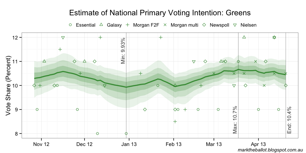
The preliminary primary vote charts from the Bayesian model follow. Please note: I am still developing and testing this analytical suite and these results should be treated with a little caution.


The observant among you will note that these four charts do not add to 100 per cent at the end point. I suspect that is the result of rounding errors (and the fact that not all of the input data from the polling houses adds to 100 per cent either).

The other thing worth noting is that while the final TPP result (see below) for a number of polling houses is similar, they way in which the primary votes add to that total is more divergent.