Further polling reflections

I have been pondering on whether the polls have been out of whack for some time, or whether it was a recent failure (over the previous 3, 6 or (say) 12 months). In previous posts, I looked at YouGov in 2017, and at monthly polling averages prior to the 2019 election.

Today I want to look at the initial polls following the 2016 election. First, however, let's recap the model I used for the 2019 election. In this model, I excluded YouGov and Roy Morgan from the sum-to-zero constraint on house effects. I have added a starting point reference to these charts (and increased the rounding on the labels from one decimal place to two. However, I would caution on reading these models to two decimal places, the models are not that precise).

What is worth noting is that this series opens on 6 July 2016 some 1.7 percentage points down from the election result of 50.36 per cent of the two-party preferred (TPP) vote for the Coalition on 2 July 2016. The series closes some 3.1 percentage points down from the 18 May 2019 election result. It appears that the core-set of Australian pollsters started some 1.7 percentage points off the mark, and collectively gained a further 1.4 percentage points of error over the period from July 2016 to May 2019.

These initial polls are all from Essential, and they are under-dispersed. (We discussed the under-dispersion problem here, here, here, and here. I will come back to this problem in a future post). The first two Newspolls were closer to the election result, but they then aligned with Essential from then on. The Newspolls from this period are also under-dispersed.

We can see how closely Newspoll and Essential tracked each other on average from the following chart of average house effects. I have Newspoll twice in this chart, based on the original method for allocating of preferences, and (Newspoll2) for the revised allocation of One Nation preferences from late in 2017.

If I had aggregated the polls prior to the 2019 election by anchoring the line to the previous election, I would have achieved a better estimate of the Coalition's performance than I did. Effectively I would have predicted a tie or a very narrow Coalition victory if I had aggregated the polls for this election with an anchor to the previous election.

A good question to ask at this point is why did I not anchor the model to the previous election? The short answer is that I have watched a number of aggregators in past election cycles use an anchored model and end up with worse predictions than those who assumed the house effects across the pollsters cancel each other out on average. I have also assumed that pollsters use elections to recalibrate their polling methodologies, and this recalibration represents a series break. A left-hand side anchored series assumes there have been no series breaks.

In summary, at least 1.7 percentage points of polling error were baked in from the very first polls following the 2016 election. Over the period since July 2016, this error has increased to 3.1 percentage points.

Wonky note: For the anchored model, I changed the priors on house effects from weakly informative normals centred on zero, to uniform priors in the range -6% to +6%. I did this because the weakly informative priors were dragging the aggregation towards the centre of the data points.

The anchored STAN model code follows.

// STAN: Two-Party Preferred (TPP) Vote Intention Model 
//     - Updated to for fixed starting point

data {
    // data size
    int n_polls;
    int n_days;
    int n_houses;
    
    // assumed standard deviation for all polls
    real pseudoSampleSigma;
    
    // poll data
    vector[n_polls] y; // TPP vote share
    int house[n_polls];
    int day[n_polls];
    //vector [n_polls] poll_qual_adj; // poll quality adjustment
    
    // period of discontinuity event
    int discontinuity;
    int stability;
    
    // previous election outcome anchor point
    real election_outcome;
}

transformed data {
    // fixed day-to-day standard deviation
    real sigma = 0.0015;
    real sigma_volatile = 0.0045;
    
    // house effect range
    real lowerHE = -0.06;
    real upperHE = 0.06;
}

parameters {
    vector[n_days] hidden_vote_share;
    vector[n_houses] pHouseEffects;
    real disruption;
}

model {
    // -- temporal model [this is the hidden state-space model]
    disruption ~ normal(0.0, 0.15); // PRIOR
    hidden_vote_share[1] ~ normal(election_outcome, 0.00001);
    
    hidden_vote_share[2:(discontinuity-1)] ~ 
        normal(hidden_vote_share[1:(discontinuity-2)], sigma);
                
    hidden_vote_share[discontinuity] ~ 
        normal(hidden_vote_share[discontinuity-1]+disruption, sigma); 

    hidden_vote_share[(discontinuity+1):stability] ~ 
        normal(hidden_vote_share[discontinuity:(stability-1)], sigma_volatile);

    hidden_vote_share[(stability+1):n_days] ~ 
        normal(hidden_vote_share[stability:(n_days-1)], sigma);
    
    // -- house effects model
    pHouseEffects ~ uniform(lowerHE, upperHE); // PRIOR 

    // -- observed data / measurement model
    y ~ normal(pHouseEffects[house] + hidden_vote_share[day], 
        pseudoSampleSigma);
}

Updated primary vote share model

For the 2019 election, I have explored a number of models for aggregating the primary vote shares, including models based on Dirichlet processes and centered logits. These older models were complicated and slow. They included constraints to ensure vote shares always summed to 100 per cent for every sample from the posterior distribution.

The model I currently run is very simple. It is based on four independent Gaussian processes for each primary vote series: Coalition, Labor, Greens and Others. In this regard it is very similar to the two-party-preferred (TPP) model.

The model has few internal constraints and it runs reasonably fast (in about 3 and half minutes). However the parameters are sampled independently, and only sum to 100 per cent in terms of the mean/median for each parameter. For the improved speed (and the absence of pesky diagnostics) this was a worthwhile compromise.

The Stan program includes a generated quantities code block in which we convert primary vote intentions to an estimated TPP vote share, based on preference flows at previous elections.

While the TPP model operates in the range 0 to 1 (with vote share values typically between 0.45 and 0.55), the new model centers all of the primary vote observations around 100. This ensures that for each party the analysis of their vote shares are well away from the edge of valid values for all model parameters. If we did not do this, the Greens vote share (often around 0.1) would be too close to the zero parameter boundary. Stan can get grumpy if it is being asked to estimate a parameter close to a boundary. 

The key outputs from the new model follow. We will start with the primary vote share aggregation and an estimate of house effects for each party.

We can compare the primary vote shares for the major and minor parties.

And we can estimate the TPP vote shares for the Coalition and Labor, based on the preference flows from previous elections

The code for the latest model is as follows.

// STAN: Primary Vote Intention Model
// Essentially a set of independent Gaussian processes from day-to-day
// for each party's primary vote, centered around a mean of 100

data {
    // data size
    int<lower=1> n_polls;
    int<lower=1> n_days;
    int<lower=1> n_houses;
    int<lower=1> n_parties;
    real<lower=0> pseudoSampleSigma;
    
    // Centreing factors 
    real<lower=0> center;
    real centreing_factors[n_parties];
    
    // poll data
    real<lower=0> centered_obs_y[n_parties, n_polls]; // poll data
    int<lower=1,upper=n_houses> house[n_polls]; // polling house
    int<lower=1,upper=n_days> poll_day[n_polls]; // day on which polling occurred

    //exclude final n parties from the sum-to-zero constraint for houseEffects
    int<lower=0> n_exclude;
    
    // period of discontinuity and subsequent increased volatility event
    int<lower=1,upper=n_days> discontinuity; // start with a discontinuity
    int<lower=1,upper=n_days> stability; // end - stability restored
    
    // day-to-day change
    real<lower=0> sigma;
    real<lower=0> sigma_volatile;

    // TPP preference flows
    vector<lower=0,upper=1>[n_parties] preference_flows_2010;
    vector<lower=0,upper=1>[n_parties] preference_flows_2013;
    vector<lower=0,upper=1>[n_parties] preference_flows_2016;
}

transformed data {
    int<lower=1> n_include = (n_houses - n_exclude);
}

parameters {
    matrix[n_days, n_parties] centre_track;
    matrix[n_houses, n_parties] pHouseEffects;
}

transformed parameters {
    matrix[n_houses, n_parties] houseEffects;
    for(p in 1:n_parties) {
        houseEffects[1:n_houses, p] = pHouseEffects[1:n_houses, p] - 
            mean(pHouseEffects[1:n_include, p]);
    }
}

model{
    for (p in 1:n_parties) {
        // -- house effects model
        pHouseEffects[, p] ~ normal(0, 8.0); // weakly informative PRIOR
        
        // -- temporal model - with a discontinuity followed by increased volatility
        centre_track[1, p] ~ normal(center, 15); // weakly informative PRIOR
        centre_track[2:(discontinuity-1), p] ~ 
            normal(centre_track[1:(discontinuity-2), p], sigma);
        centre_track[discontinuity, p] ~ normal(center, 15); // weakly informative PRIOR
        centre_track[(discontinuity+1):stability, p] ~ 
            normal(centre_track[discontinuity:(stability-1), p], sigma_volatile);
        centre_track[(stability+1):n_days, p] ~ 
            normal(centre_track[stability:(n_days-1), p], sigma);

        // -- observational model
        centered_obs_y[p,] ~ normal(houseEffects[house, p] + 
            centre_track[poll_day, p], pseudoSampleSigma);
    }
}

generated quantities {
    matrix[n_days, n_parties]  hidden_vote_share;
    vector [n_days] tpp2010;
    vector [n_days] tpp2013;
    vector [n_days] tpp2016;
    
    for (p in 1:n_parties) {
        hidden_vote_share[,p] = centre_track[,p] - centreing_factors[p];
    }
    
    // aggregated TPP estimates based on past preference flows
    for (d in 1:n_days){
        // note matrix transpose in next three lines
        tpp2010[d] = sum(hidden_vote_share'[,d] .* preference_flows_2010);
        tpp2013[d] = sum(hidden_vote_share'[,d] .* preference_flows_2013);
        tpp2016[d] = sum(hidden_vote_share'[,d] .* preference_flows_2016);
    }
} 

The Python program to run this Stan model follows. 

# PYTHON: analyse primary poll data

import pandas as pd
import numpy as np
import pystan
import pickle

import sys
sys.path.append( '../bin' )
from stan_cache import stan_cache

# --- check version information
print('Python version: {}'.format(sys.version))
print('pystan version: {}'.format(pystan.__version__))

# --- curate the data for the model
# key settings
intermediate_data_dir = "./Intermediate/" # analysis saved here

# preference flows
parties  =              ['L/NP', 'ALP', 'GRN', 'OTH']
preference_flows_2010 = [0.9975, 0.0, 0.2116, 0.5826]
preference_flows_2013 = [0.9975, 0.0, 0.1697, 0.5330]
preference_flows_2016 = [0.9975, 0.0, 0.1806, 0.5075]
n_parties = len(parties)

# polling data
workbook = pd.ExcelFile('./Data/poll-data.xlsx')
df = workbook.parse('Data')

# drop pre-2016 election data
df['MidDate'] = [pd.Period(d, freq='D') for d in df['MidDate']]
df = df[df['MidDate'] > pd.Period('2016-07-04', freq='D')] 

# push One Nation into Other 
df['ONP'] = df['ONP'].fillna(0)
df['OTH'] = df['OTH'] + df['ONP']

# set start date
start = df['MidDate'].min() - 1 # the first date is day 1
df['Day'] = df['MidDate'] - start # day number for each poll
n_days = df['Day'].max() # maximum days 
n_polls = len(df)

# set discontinuity date - Turnbull's last day in office
discontinuity = pd.Period('2018-08-23', freq='D') - start # UPDATE
stability = pd.Period('2018-10-01', freq='D') - start # UPDATE


# manipulate polling data ... 
y = df[parties]
center = 100
centreing_factors = center - y.mean()
y = y + centreing_factors

# add polling house data to the mix
# make sure the "sum to zero" exclusions are 
# last in the list
houses = df['Firm'].unique().tolist()
exclusions = ['YouGov', 'Ipsos']
# Note: we are excluding YouGov and Ipsos 
# from the sum to zero constraint because 
# they have unusual poll results compared 
# with other pollsters
for e in exclusions:
    assert(e in houses)
    houses.remove(e)
houses = houses + exclusions
map = dict(zip(houses, range(1, len(houses)+1)))
df['House'] = df['Firm'].map(map)
n_houses = len(df['House'].unique())
n_exclude = len(exclusions)

# sample metrics
sampleSize = 1000 # treat all polls as being of this size
pseudoSampleSigma = np.sqrt((50 * 50) / sampleSize) 

# --- compile model

# get the STAN model 
with open ("./Models/primary simultaneous model.stan", "r") as f:
    model = f.read()
    f.close()

# encode the STAN model in C++ 
sm = stan_cache(model_code=model)


# --- fit the model to the data
ct_init = np.full([n_days, n_parties], center*1.0)
def initfun():
    return dict(centre_track=ct_init)

chains = 5
iterations = 2000
data = {
        'n_days': n_days,
        'n_polls': n_polls,
        'n_houses': n_houses,
        'n_parties': n_parties,
        'pseudoSampleSigma': pseudoSampleSigma,
        'centreing_factors': centreing_factors,
    
        'centered_obs_y': y.T, 
        'poll_day': df['Day'].values.tolist(),
        'house': df['House'].values.tolist(), 
        'n_exclude': n_exclude,
        'center': center,
        'discontinuity': discontinuity,
        'stability': stability,
        
        # let's set the day-to-day smoothing 
        'sigma': 0.15,
        'sigma_volatile': 0.4,
        
        # preference flows at past elections
        'preference_flows_2010': preference_flows_2010,
        'preference_flows_2013': preference_flows_2013,
        'preference_flows_2016': preference_flows_2016
}
    
fit = sm.sampling(data=data, iter=iterations, chains=chains, 
    init=initfun, control={'max_treedepth':13})
results = fit.extract()

# --- check diagnostics
print('Stan Finished ...')
import pystan.diagnostics as psd
print(psd.check_hmc_diagnostics(fit))

# --- save the analysis
with open(intermediate_data_dir + 'cat-' +
    'output-primary-zero-sum.pkl', 'wb') as f:
    pickle.dump([df,sm,fit,results,data,
        centreing_factors, exclusions], f)
    f.close()

Polling update

Today we had an Ipsos poll (45-55 in Labor's favour) and a Newspoll (47-53) with vastly different interpretations. For Newspoll the story was one of steady Coalition improvement (47 is better than Morrison's debut at 44). For Ipsos it was one of no benefit from the recent leadership change. The last Turnbull poll under Ipsos was also 45-55.

In the Bayesian model, I have allowed for a discontinuity in public opinion on 23 August, and for a period of higher than normal volatility in day-to-day voting sentiment from 24 August to 1 October. The results are as follows.

Enough time has passed since the Coalition leadership change for the moving average models to start to come back into alignment with the Bayesian model. Not withstanding the Coalition bounce following the immediate polling collapse in reaction to the leadership change in August 2018, Coalition voting sentiment is as low now as it was at Turnbull's worst period in the polls in late 2017.

My primary vote model has decided to stop working. Actually, I upgraded to the latest versions of Stan and pystan, and I need to tweak the model to get it working again.

Model updates are coming

The change of party leader necessitates the introduction of a discontinuity in the model associated with the transition from Prime Minister Turnbull to Prime Minister Morrison. Because the current model is written in Stan, the process is similar but subtly different from when I did similar things for Rudd to Gillard, Gillard to Rudd, and Abbot to Turnbull; all back in the day when I was modelling in JAGS.

I have also taken the opportunity to repair an element of the model that has nagged at me. Because the polling data is relatively sparse compared with the unit of temporal analysis (days), the derived standard deviation on the day-to-day changes in the model can be under-estimated. Rather than have the model estimate this factor (typically with a median estimate at 0.0007 of the two-party preferred (TPP) vote-share), I have specified a standard deviation on day-to-day changes in the vote share of 0.002. For reference, 100 per cent of the vote-share is represented in the model with the number one.

At the conclusion of the Turnbull government, the TPP model follows. This model has a specified standard deviation on the day-to-day change in vote share set to 0.002.

We can compare this with the moving averages below.

It is arguable that the last poll in the series was an outlier: Ipsos at 45 per cent for the Coalition over the period 15-18 August. Most recent polls had the Coalition on 49 per cent. As the final poll in the series, it has affected the Bayesian analysis more than it has the moving averages. If we re-run the analysis without that final poll, the Turnbull trajectory for the past 9 months has been strong, and a win at the next election for the Coalition did not look inconceivable, even should the trend have continued at a slower rate from now. Obviously, the current polls still had Labor ahead, but with the Coalition recovering lost ground over much of the year to date.

Turning to the primary vote model, I have made a similar adjustment to the standard deviation on day-to-day changes in voting intention. This time from a model derived 0.003 to an imposed 0.009. The unit of analysis for this is less intuitive, being on the centered logit scale, which is highly non-linear. The results follow.

The implied TPP results follow ... they don't have the same drop associated with the most recent Ipsos poll.

I am working on the revised models for when new poll results under the Morrison leadership are released. My updated code for the two models follows. This code provides for a discontinuity- but it is still in a development and test cycle - so not yet finalised.

// STAN: Two-Party Preferred (TPP) Vote Intention Model 
//     - Updated to allow for a discontinuity event. 

data {
    // data size
    int n_polls;
    int n_days;
    int n_houses;
    
    // assumed standard deviation for all polls
    real pseudoSampleSigma;
    
    // we are only going to normalise house effects from first n houses
    int n_core_set;
    
    // poll data
    vector[n_polls] y; // TPP vote share
    int house[n_polls];
    int day[n_polls];
    
    // day of discontinuity event
    int discontinuity;
}

transformed data {
    // Specify sigma in this block if you do not 
    // want the model to derive a value for 
    // the standard deviation on day-to-day
    // changes in the value of hidden_vote_share
    // NOTE: Also requres changes in parameters and 
    // model blocks below.
    
    real sigma = 0.0015;
    
    // Technical note: smaller values of sigma produce 
    // smoother (but less responsive) lines of analysis. 
    // Technical note: because the poll data is relatively 
    // sparse compared with the temporal unit of analysis 
    // (days), the model derived sigma will be understated. 
    // Technical note: from July 16 to July 18 the median 
    // model derived sigma was 0.0007
}

parameters {
    vector[n_days] hidden_vote_share; 
    vector[n_houses] pHouseEffects;
    
    // speicfy sigma here for a model derived value
    //real sigma; // SD of day-to-day change 
}

transformed parameters {
    vector[n_houses] houseEffect;
    
    // house effects sum to zero over the first n_core_set houses
    // this allows you to specify a "trusted" set of pollsters
    
    houseEffect[1:n_core_set] = pHouseEffects[1:n_core_set] - 
        mean(pHouseEffects[1:n_core_set]);
    if(n_core_set < n_houses)
        houseEffect[(n_core_set+1):n_houses] = 
            pHouseEffects[(n_core_set+1):n_houses];
}

model {
    // -- temporal model [this is the hidden state-space model]
    
    // - comment out the next line if sigma is not model derived
    // sigma ~ cauchy(0, 0.0025); // half cauchy prior
    
    // - hidden daily voting intention 
    // NOTE: the priors for the temporal model of hidden voting 
    // intention are weakly informative and therefore should be 
    // selected with some reference to the subsequent data
    hidden_vote_share[1] ~ normal(0.49, 0.0333); // PRIOR
    // update for discontinuity follows
    //hidden_vote_share[2:n_days] ~ 
    //    normal(hidden_vote_share[1:(n_days-1)], sigma);
    hidden_vote_share[discontinuity] ~ normal(0.44, 0.0333); // PRIOR
    hidden_vote_share[2:(discontinuity-1)] ~ 
        normal(hidden_vote_share[1:(discontinuity-2)], sigma);
    hidden_vote_share[(discontinuity+1):n_days] ~ 
        normal(hidden_vote_share[discontinuity:(n_days-1)], sigma);
    
    // -- house effects model
    
    pHouseEffects ~ normal(0, 0.025); // up to +/- 5 percentage points 

    // -- observed data / measurement model
    
    y ~ normal(houseEffect[house] + 
        hidden_vote_share[day], pseudoSampleSigma);
}

// STAN: Primary Vote Intention Model using Centred Logits
//     - Updated to handle the Turnbull to Morrison discontinuity
//     - Updated to use a specified standard deviation on 
//       day-to-day voting intentions.

data {
    // data size
    int<lower=1> n_polls;
    int<lower=1> n_days;
    int<lower=1> n_houses;
    int<lower=1> n_parties;
    int<lower=1> pseudoSampleSize;
    
    // Centreing factors 
    real centreing_factors[n_parties]; // Updated 
    
    // poll data - provided in three variables
    // y in the next line is effectively an array of multinomials
    int<lower=1,upper=pseudoSampleSize> y[n_polls, n_parties]; 
    int<lower=1,upper=n_houses> house[n_polls]; // polling house
    int<lower=1,upper=n_days> poll_day[n_polls]; // day poll taken
    
    // TPP preference flows from previous elections
    row_vector<lower=0,upper=1>[n_parties] preference_flows_2010;
    row_vector<lower=0,upper=1>[n_parties] preference_flows_2013;
    row_vector<lower=0,upper=1>[n_parties] preference_flows_2016;
    
    // day of discontinuity event (from Turnbull to Morrison)
    int<lower=1,upper=n_days> discontinuity;
}

transformed data {
    // NOTE: Specify sigma in this block if you 
    // do not want the model to derive a value 
    // for the standard deviation on day-to-day
    // changes in the value of hidden_vote_share
    // NOTE: Also requires changes in parameters and 
    // model blocks below.
    
    real sigma = 0.009; // Note: logit scale near the origin
    
    // Note: median model derived from Jul-16 to Ju-18 was 
    // around 0.003. 
}
 
parameters {
    // NOTE: because the vote-share from four parties
    // sums to one, we only need to model three as
    // centred logits. We can derive the four party
    // simplex from the three modeled logits
    row_vector[n_days] centredLogits[n_parties-1];
    matrix[n_houses-1, n_parties-1] houseAdjustment;

    // comment next line if model is not finding sigma
    //real<lower=0> sigma; 
}

transformed parameters {
    matrix[n_parties, n_days] hidden_voting_intention; // simplex
    vector<lower=-0.2,upper=0.2>[n_parties] tHouseAdjustment[n_houses];
    row_vector[n_days] tmp; // tmp var used to find the redundant party
    
    // -- house effects - two-direction sum to zero constraints
    for (h in 1:(n_houses-1)) {
        for(p in 1:(n_parties-1)) {
            tHouseAdjustment[h][p] = houseAdjustment[h][p];
        }
    }
    for(p in 1:(n_parties-1)) {
        tHouseAdjustment[n_houses][p] = -sum(col(houseAdjustment, p));
    }
    for(h in 1:n_houses) {
        tHouseAdjustment[h][n_parties] = 0; // get rid of the NAN
        tHouseAdjustment[h][n_parties] = -sum(tHouseAdjustment[h]);
    }
    
    // -- convert centred logits to a simplex of hidden voting intentions
    tmp = rep_row_vector(0, n_days);
    for (p in 1:(n_parties-1)) {
        hidden_voting_intention[p] = inv_logit(centredLogits[p]) + 
            centreing_factors[p];
        tmp = tmp + hidden_voting_intention[p];
    }
    hidden_voting_intention[n_parties] = 1.0 - tmp; 
}

model{
    matrix[n_parties, n_polls] hvi_on_poll_day;

    // -- house effects model
    
    for( h in 1:(n_houses-1) ) {
        houseAdjustment[h] ~ normal(0, 0.015); 
    }
    
    // -- temporal model - [AKA the hidden state-space model]
 
    // - day-to-day standard deviation
    // Note: 0.02 near the centre --> roughly std dev of half a per cent 
    // Comment out the next line if you do not want the model to find sigma
    //sigma ~ normal(0, 0.02); // half normal prior - note: on logit scale;

    // - AR(1) temporal model with a discontinuity
    for(p in 1:(n_parties-1)) { 
        // centred starting point 50% +/- 5% = zero on the logit scale
        centredLogits[p][1] ~ normal(0, 0.15); 
        //centredLogits[p][2:n_days] ~ 
        //  normal(centredLogits[p][1:(n_days-1)], sigma);
        
        // - update for discontinuity
        centredLogits[p][discontinuity] ~ normal(0, 0.15);
        centredLogits[p][2:(discontinuity-1)] ~ 
            normal(centredLogits[p][1:(discontinuity-2)], sigma);
        centredLogits[p][(discontinuity+1):n_days] ~ 
            normal(centredLogits[p][discontinuity:(n_days-1)], sigma);
    }
    
    // -- observed data model [AKA the measurement model]
    
    for(p in 1:n_parties) {
        hvi_on_poll_day[p] = hidden_voting_intention[p][poll_day];
    }
    for(poll in 1:n_polls) {
        // note matrix transpose in the next statement ...
        y[poll] ~ multinomial(to_vector(hvi_on_poll_day'[poll]) + 
            tHouseAdjustment[house[poll]]);
    }
}

generated quantities {
    // aggregated TPP estimates based on past preference flows
    vector [n_days] tpp2010;
    vector [n_days] tpp2013;
    vector [n_days] tpp2016;

    for (d in 1:n_days){
        // note matrix transpose in next three lines
        tpp2010[d] = sum(hidden_voting_intention'[d] .* 
            preference_flows_2010);
        tpp2013[d] = sum(hidden_voting_intention'[d] .* 
            preference_flows_2013);
        tpp2016[d] = sum(hidden_voting_intention'[d] .* 
            preference_flows_2016);
    }
}

Pollster preference flows

One of the things I like to look at is the preference flows the pollsters apply to their primary vote estimates in order to make a two-party preferred (TPP) vote estimate. We can discover these flows using good old fashioned multiple linear regression, along these lines:

$$TPP - Coalition_p = \beta_1 Greens_p + \beta_2 OneNation_p + \beta_3 Other_p + \epsilon$$

Which, in matrix notation, we will simplify as:

$$ y = X \beta + \epsilon $$

In this simplification, \(y\) is a column vector of (TPP - Coalition primary) vote estimates from a pollster. \(X\) is the regression design matrix, with k columns (one for each party's primary vote) and N rows (one for each of the reported poll results). \(\beta\) is a column vector of party coefficients we are seeking to find through the regression process. And \(\epsilon\) is a column vector of error terms which we assume are independent and identically distributed (iid) with a mean of \(0\). Through the magic of mathematics we can seek to minimize the sum of the squared errors using algebra and calculus to show:

$$ \sum_{i=1}^n\epsilon_i^2 = \epsilon'\epsilon = (y-X\beta)'(y-X\beta) $$
$$= y'y - \beta'X'y - y'X\beta + \beta'X'X\beta $$
$$= y'y - 2\beta'X'y + \beta'X'X\beta $$
From this last equation, we can use calculus to find the \(\beta\) that minimizes the sum of the errors squared:
$$\frac{\partial \epsilon'\epsilon}{\partial\beta} = -2X'y+2X'X\beta = 0$$
Which can be re-arranged to the famous "ex prime ex inverse ex prime why":
$$ \beta = (X'X)^{-1}X'y $$

Before I get to the results, there are a few caveats to go through. First, not all of the primary vote poll data sums to 100 per cent. In the data I looked at, the following polls did not sum to 100 per cent.

--- Does not add to 100% ---
     L/NP   ALP   GRN   ONP   OTH    Sum       Firm            Date
12   35.0  38.0  10.0   7.0   9.0   99.0  Essential     12 Dec 2017
18   31.0  34.0  11.0  11.0  14.0  101.0     YouGov     14 Nov 2017
19   36.0  38.0   9.0   8.0  10.0  101.0  Essential     14 Nov 2017
21   36.0  37.0  10.0   7.0   9.0   99.0  Essential     30 Oct 2017
25   36.0  38.0  10.0   7.0  10.0  101.0  Essential      4 Oct 2017
32   35.0  34.0  14.0   1.0  15.0   99.0      Ipsos    6-9 Sep 2017
63   36.0  37.0  10.0   8.0  10.0  101.0  Essential  13-16 Apr 2017
67   35.0  37.0  10.0   8.0  11.0  101.0  Essential  24-27 Mar 2017
69   34.0  37.0   9.0  10.0   9.0   99.0  Essential  17-20 Mar 2017
75   36.0  35.0   9.0  10.0   9.0   99.0  Essential   9-12 Feb 2017
77   35.0  37.0  10.0   9.0   8.0   99.0  Essential  20-23 Jan 2017
80   37.0  37.0   9.0   7.0   9.0   99.0  Essential   9-12 Dec 2016
83   36.0  30.0  16.0   7.0   9.0   98.0      Ipsos  24-26 Nov 2016
88   37.0  37.0  11.0   5.0   9.0   99.0  Essential  14-17 Oct 2016
92   38.0  37.0  10.0   5.0  11.0  101.0  Essential   9-12 Sep 2016
109  34.0  35.0  11.0   8.0  13.0  101.0     YouGov   7-10 Dec 2017
110  32.0  32.0  10.0  11.0  16.0  101.0     YouGov  23-27 Nov 2017
----------------------------

To manage this, I normalised all of the primary vote poll results so that they summed to 1. 

The second thing I did was limit my analysis to those pollsters that had more than 10 polls since the last election. This meant I limited my analysis to polls from Newspoll and Essential.

Let's look at the multiple regression results. The key results is the block in the middle, with the three parties in the left hand column: GRN, ONP and OTH - Greens, One Nation and Others. The first coefficient column is the best linear unbiased estimate of the preference flows to the Coalition from each of these parties. The 95 per cent confidence intervals can be seen in the far right columns.

---- Essential ----
                            OLS Regression Results                            
==============================================================================
Dep. Variable:                      y   R-squared:                       0.999
Model:                            OLS   Adj. R-squared:                  0.999
Method:                 Least Squares   F-statistic:                 1.173e+04
Date:                Sat, 17 Mar 2018   Prob (F-statistic):           2.09e-61
Time:                        13:12:35   Log-Likelihood:                 190.20
No. Observations:                  45   AIC:                            -374.4
Df Residuals:                      42   BIC:                            -369.0
Df Model:                           3                                         
Covariance Type:            nonrobust                                         
==============================================================================
                 coef    std err          t      P>|t|      [0.025      0.975]
------------------------------------------------------------------------------
GRN            0.2236      0.054      4.162      0.000       0.115       0.332
ONP            0.4396      0.037     11.775      0.000       0.364       0.515
OTH            0.5091      0.050     10.190      0.000       0.408       0.610
==============================================================================
Omnibus:                        3.681   Durbin-Watson:                   1.938
Prob(Omnibus):                  0.159   Jarque-Bera (JB):                1.691
Skew:                          -0.020   Prob(JB):                        0.429
Kurtosis:                       2.051   Cond. No.                         20.0
==============================================================================

---- Newspoll ----
                            OLS Regression Results                            
==============================================================================
Dep. Variable:                      y   R-squared:                       0.999
Model:                            OLS   Adj. R-squared:                  0.999
Method:                 Least Squares   F-statistic:                     7414.
Date:                Sat, 17 Mar 2018   Prob (F-statistic):           1.81e-34
Time:                        13:12:38   Log-Likelihood:                 110.81
No. Observations:                  26   AIC:                            -215.6
Df Residuals:                      23   BIC:                            -211.9
Df Model:                           3                                         
Covariance Type:            nonrobust                                         
==============================================================================
                 coef    std err          t      P>|t|      [0.025      0.975]
------------------------------------------------------------------------------
GRN            0.2581      0.090      2.881      0.008       0.073       0.443
ONP            0.4976      0.035     14.202      0.000       0.425       0.570
OTH            0.4424      0.084      5.237      0.000       0.268       0.617
==============================================================================
Omnibus:                        2.886   Durbin-Watson:                   0.753
Prob(Omnibus):                  0.236   Jarque-Bera (JB):                1.437
Skew:                          -0.212   Prob(JB):                        0.488
Kurtosis:                       1.929   Cond. No.                         26.8
==============================================================================

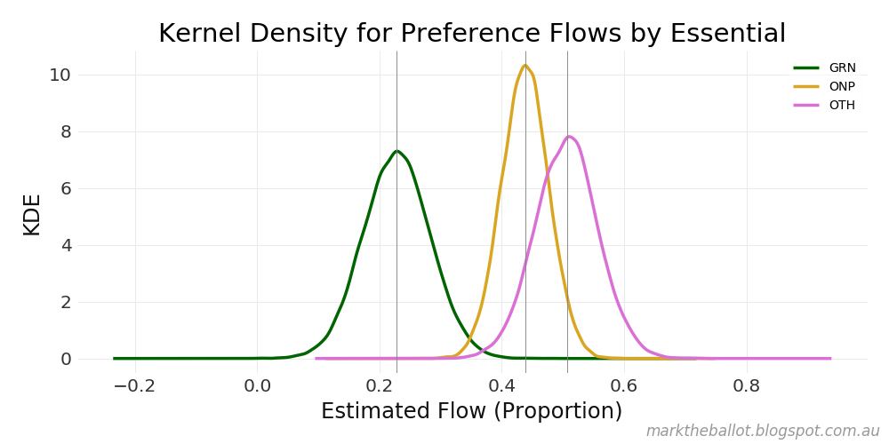
From the Ordinary Least Squares (OLS) multiple regression analysis, our best guess is that Essential flows 22 per cent of the Green vote to the Coalition, it flows 44 per cent of the One Nation vote, and it flows 51 per cent of the Other vote. In comparison, Newspoll flows 26 per cent of the Green vote to the Coalition, 50 per cent of the One Nation vote, and 44 per cent of the Other vote.

While we get an estimate of preference flows to the Coalition for each of the three parties from both pollsters, it is worth noting that small sample sizes have resulted in quite wide confidence intervals for these estimates.

We can also do a Bayesian multiple linear regression. The Stan model I used for this follows.

// STAN: multiple regression - no intercept - positive coefficients

data {
    // data size
    int<lower=1> k;                     // number of pollster firms
    int<lower=k+1> N;                   // number of polls

    vector<lower=0,upper=1>[N] y;       // response vector
    matrix<lower=0,upper=1>[N, k] X;    // design matrix
}

parameters {
    vector<lower=0>[k] beta;    // positive regression coefficients
    real<lower=0> sigma;        // standard deviation on iid error term
}

model {
    beta ~ normal(0, 0.5);      // half normal prior
    sigma ~ cauchy(0, 0.01);    // half cauchy prior
    y ~ normal(X * beta, sigma);// regression model
}

The results I got were very similar to the standard OLS results. In this case I have identified the 95% credible interval, which is the Bayesian equivalent of the confidence interval. Again, the One Nation and Other results are quite different, and swapped about between the two pollsters.

From Stan: for Essential
           2.5%    median     97.5%
GRN    0.121745  0.228054  0.335852
ONP    0.362631  0.438261  0.513884
OTH    0.404663  0.506283  0.607355

From Stan: for Newspoll
           2.5%    median     97.5%
GRN    0.089876  0.267659  0.450531
ONP    0.420720  0.494935  0.566663
OTH    0.259106  0.433838  0.601585

From the Bayesian analysis, our best guess is that Essential flows 23 per cent of the Green vote to the Coalition. It flows 44 per cent of the One Nation vote. And it flows 51 per cent of the Other vote. In comparison, Newspoll flows 27 per cent of the Green vote to the Coalition, 49 per cent of the One Nation vote, and 43 per cent of the Other vote.

These Bayesian results can be charted as probability densities as follows. In these charts the median sample for each distribution is highlighted with a thin vertical line.

For completeness, the supporting Python program that generated this analysis follows.

# PYTHON - estimates of preference flows from polling data

import pandas as pd
import numpy as np
import statsmodels.api as sm
import matplotlib.pyplot as plt

import sys
sys.path.append( '../bin' )
from stan_cache import stan_cache

# --- chart results
graph_dir = './Graphs/'
walk_leader = 'STAN-PREFERENCE-FLOWS-'
plt.style.use('../bin/markgraph.mplstyle')

# --- curate data for analysis
workbook = pd.ExcelFile('./Data/poll-data.xlsx')
df = workbook.parse('Data')

# drop polls without one nation 
df = df[df['ONP'].notnull()]

# drop pre-2016 election data
df['MidDate'] = [pd.Period(d, freq='D') for d in df['MidDate']]
df = df[df['MidDate'] > pd.Period('2016-07-04', freq='D')] 

# normalise the data - still in 0 to 100 range
parties = ['GRN', 'ONP', 'OTH']
all = ['L/NP', 'ALP'] + parties
df['Sum'] = df[all].sum(axis=1)
bad = df[all + ['Sum', 'Firm', 'Date']]
bad = bad[(bad['Sum'] < 99.5) | (bad['Sum'] > 100.5)]
print('--- Does not add to 100% ---')
print(bad)
print('----------------------------')
df[all] = df[all].div(df[all].sum(axis=1), axis=0) * 100.0

# --- Analyse the curated data 
firms = df['Firm'].unique()
for firm in firms:
    cases = df[df['Firm']==firm]
    
    if len(cases) <= 10:
        continue # not enough to analyse
    
    # --- classic OLS multiple regression
    # get response vector and design matrix in 0 to 1 range 
    y = (cases['TPP L/NP'] - cases['L/NP']) / 100.0 
    X = cases[parties] / 100.0
    
    # regression estimation
    model = sm.OLS(y, X).fit()
    print('\n\n---- {} ----'.format(firm))
    # Print out the statistics
    print(model.summary())
    
    # --- let's do the same thing with Stan
    # input data
    data = {
        'y': y,
        'X' : X,
        'N': len(y),
        'k': len(X.columns)
    }
    
    # helpers
    quants = [2.5,  50, 97.5]
    labels = ['2.5%', 'median', '97.5%']
    
    with open ("./Models/preference flows.stan", "r") as file:
        model_code = file.read()
        file.close()
        
        # model
        stan = stan_cache(model_code=model_code, model_name='preference flows')
        fit = stan.sampling(data=data, iter=10000, chains=5)
        results = fit.extract()

        # capture the coefficients
        coefficients = results['beta']
        print('--- Coefficient Shape: {} ---'.format(coefficients.shape))
        estimates = pd.DataFrame()
        for i, party in zip(range(len(parties)), parties):
            q = np.percentile(coefficients[:,i], quants)
            row = pd.DataFrame(q, index=labels, columns=[party]).T
            estimates = estimates.append(row)

        # capture sigma
        sigma = results['sigma'].T
        q = np.percentile(sigma, quants)
        row = pd.DataFrame(q, index=labels, columns=['sigma']).T
        estimates = estimates.append(row)
        
        # print results from Stan
        print('From Stan: for {}'.format(firm))
        print(estimates)
        
        # plot results from Stan
        coefficients = pd.DataFrame(coefficients, columns=parties)
        ax = coefficients.plot.kde(color=['darkgreen', 'goldenrod', 'orchid']) 
        ax.set_title('Kernel Density for Preference Flows by {}'.format(firm))
        ax.set_ylabel('KDE')
        ax.set_xlabel('Estimated Flow (Proportion)')
        for i in coefficients.columns:
            ax.axvline(x=coefficients[i].median(), color='gray', linewidth=0.5)

        fig = ax.figure
        fig.set_size_inches(8, 4)
        fig.tight_layout(pad=1)
        fig.text(0.99, 0.01, 'marktheballot.blogspot.com.au',
            ha='right', va='bottom', fontsize='x-small', 
            fontstyle='italic', color='#999999') 
        fig.savefig(graph_dir+walk_leader+firm+'.png', dpi=125) 
        plt.close() 

What do you do when the data does not fit the model?

I have a couple of models in development for aggregating primary vote intention. I thought I would extend the centred logit model from four parties (Coalition, Labor, Greens and Other) to five parties (Coalition, Labor, Greens, One Nation and Other). It was not a significant change to the model. However, when I went to run it, it generated pages of warning messages, well into the warm-up cycle:

The current Metropolis proposal is about to be rejected because of the following issue:[boring technical reason deleted]

If this warning occurs sporadically, such as for highly constrained variable types like covariance matrices, then the sampler is fine, but if this warning occurs often then your model may be either severely ill-conditioned or misspecified.

My model is highly constrained, and it would produce a few of these warnings at start-up. But it was nothing like the number now being produced. Fortunately, the model was not completely broken, and it did produce an estimate.

When I looked at the output from the model, the issue was immediately evident: the Ipsos data was inconsistent with the assumptions in my model. In this chart, the first Ipsos poll result for One Nation is close to the results from the other pollsters. But the remaining three polls are well below the estimate from the other pollsters. This difference delivers a large house bias estimate for Ipsos, well to the edge of my prior for house biases: normal(0, 0.015) - ie. a normal distribution with a mean of 0 and a standard deviation of 1.5 per percentage points.

The model assumes that each polling house will track around some hidden population trend, with each poll's deviation from that trend being explained by two factors: a random amount associated with the sampling variation, and a constant additive amount associated with the systemic house bias for that pollster.

If we assume the other pollsters are close to the trend, then a few explanations are possible (listed in my ranking of higher to lower plausibility):

• Ipsos changed its polling methodology between the first and subsequent polls, and the model's assumption of a constant additive systemic house bias is incorrect; or
• the first poll is a huge outlier for Ipsos (well outside of the typical variation associated with the sampling variation from each poll), and the remaining three polls are more typical and incorporate a substantial house bias for Ipsos; or
• the first Ipsos poll is more plausible for Ipsos, and the last three are huge outliers.

Whatever, it makes the resolution of an estimate more challenging for Stan. And it gives me something more to ponder.

I should note that while the Ipsos results are low for One Nation, they are consistently above average for the Greens. Being consistently above is in line with model assumptions.

There is some allure in removing the Ipsos data from the model; but there be dragons. As a general rule of thumb, removing outliers from the data requires a compelling justification, such as independent verification of a measurement error. I like to think of outliers as a disturbance in the data where I don't yet know/understand what causes that disturbance.

March 2018 polling update

I have been busy coding a new primary vote aggregation model in Stan and Python. It was an interesting experience as I came to terms with the way in which Stan differs from JAGS (and the ways in which the Hamiltonian Monte Carlo sampling differs from Gibbs sampling). While I found Stan a little more fiddly to code, it is definitely easier to debug, requires fewer iterations, and is therefore faster to both code and run. I will write a technical post shortly on the primary vote aggregation model, as well as some of my experiences with Stan.

So let's get down to the data. First, however, an acknowledgement: I sourced the polling data from the Wikipedia page on the next Australian federal election.

The two-party preferred (TPP) aggregation tends to significant levels of smoothing. At the start of March this model estimates the Coalition would win 47.3 per cent of the TPP vote share. While I have not converted this to an election outcome probability (the next task), this result is strongly suggestive of sizable Labor win, were an election held at the moment.

Next we will look at the primary vote aggregation model I have just completed. This model is not as smoothed as the TPP aggregation model. It is more sensitive to week-on-week polling changes. It is an interesting question whether this is just picking up noise or better listening to the underlying signal.

Of note is the recent decline in primary vote share for Labor and the Coalition. These votes have moved to the Greens and the other parties.

The above charts can be summarised and compared as follows:

The house adjustments are more complicated than for the TPP model. The sum to zero constraint needs to be maintained in two directions simultaneously: for each pollster across the four party groups; and for each party, across the (currently) five pollsters in the data. It is this two-way necessity that sees the median lines sometime appear to sit above or below the preponderance of polling results.

For the primary vote estimates we can calculate a TPP estimate using the preference flows evidenced at the previous election. In this model, I attribute the Other vote share in a single transfer. I do this using the preference flows from the previous elections. Pollsters can be more nuanced because they capture the specific other party from their respondents. They can then apply the actual previous election preference transfer rate for the specific primary party vote nominated by the respondent. [Another acknowledgement: I used Antony Green's reporting on preference flows].

Of note: when the polls are suggesting almost 30 per cent of the primary vote is not going to the major Coalition and Labor parties, how preferences flow will substantially shape the final election outcome. There is a 1.7 percentage point difference in the final TPP estimate between the application of the 2010 and 2016 preference flows.

This can be summarised as follows.