$$TPP - Coalition_p = \beta_1 Greens_p + \beta_2 OneNation_p + \beta_3 Other_p + \epsilon$$
Which, in matrix notation, we will simplify as:
$$ y = X \beta + \epsilon $$
In this simplification, \(y\) is a column vector of (TPP - Coalition primary) vote estimates from a pollster. \(X\) is the regression design matrix, with k columns (one for each party's primary vote) and N rows (one for each of the reported poll results). \(\beta\) is a column vector of party coefficients we are seeking to find through the regression process. And \(\epsilon\) is a column vector of error terms which we assume are independent and identically distributed (iid) with a mean of \(0\). Through the magic of mathematics we can seek to minimize the sum of the squared errors using algebra and calculus to show:
$$ \sum_{i=1}^n\epsilon_i^2 = \epsilon'\epsilon = (y-X\beta)'(y-X\beta) $$
$$= y'y - \beta'X'y - y'X\beta + \beta'X'X\beta $$
$$= y'y - 2\beta'X'y + \beta'X'X\beta $$
From this last equation, we can use calculus to find the \(\beta\) that minimizes the sum of the errors squared:
$$\frac{\partial \epsilon'\epsilon}{\partial\beta} = -2X'y+2X'X\beta = 0$$
Which can be re-arranged to the famous "ex prime ex inverse ex prime why":
$$ \beta = (X'X)^{-1}X'y $$
Before I get to the results, there are a few caveats to go through. First, not all of the primary vote poll data sums to 100 per cent. In the data I looked at, the following polls did not sum to 100 per cent.
--- Does not add to 100% ---
     L/NP   ALP   GRN   ONP   OTH    Sum       Firm            Date
12   35.0  38.0  10.0   7.0   9.0   99.0  Essential     12 Dec 2017
18   31.0  34.0  11.0  11.0  14.0  101.0     YouGov     14 Nov 2017
19   36.0  38.0   9.0   8.0  10.0  101.0  Essential     14 Nov 2017
21   36.0  37.0  10.0   7.0   9.0   99.0  Essential     30 Oct 2017
25   36.0  38.0  10.0   7.0  10.0  101.0  Essential      4 Oct 2017
32   35.0  34.0  14.0   1.0  15.0   99.0      Ipsos    6-9 Sep 2017
63   36.0  37.0  10.0   8.0  10.0  101.0  Essential  13-16 Apr 2017
67   35.0  37.0  10.0   8.0  11.0  101.0  Essential  24-27 Mar 2017
69   34.0  37.0   9.0  10.0   9.0   99.0  Essential  17-20 Mar 2017
75   36.0  35.0   9.0  10.0   9.0   99.0  Essential   9-12 Feb 2017
77   35.0  37.0  10.0   9.0   8.0   99.0  Essential  20-23 Jan 2017
80   37.0  37.0   9.0   7.0   9.0   99.0  Essential   9-12 Dec 2016
83   36.0  30.0  16.0   7.0   9.0   98.0      Ipsos  24-26 Nov 2016
88   37.0  37.0  11.0   5.0   9.0   99.0  Essential  14-17 Oct 2016
92   38.0  37.0  10.0   5.0  11.0  101.0  Essential   9-12 Sep 2016
109  34.0  35.0  11.0   8.0  13.0  101.0     YouGov   7-10 Dec 2017
110  32.0  32.0  10.0  11.0  16.0  101.0     YouGov  23-27 Nov 2017
----------------------------
To manage this, I normalised all of the primary vote poll results so that they summed to 1.
The second thing I did was limit my analysis to those pollsters that had more than 10 polls since the last election. This meant I limited my analysis to polls from Newspoll and Essential.
Let's look at the multiple regression results. The key results is the block in the middle, with the three parties in the left hand column: GRN, ONP and OTH - Greens, One Nation and Others. The first coefficient column is the best linear unbiased estimate of the preference flows to the Coalition from each of these parties. The 95 per cent confidence intervals can be seen in the far right columns.
---- Essential ----
                            OLS Regression Results
==============================================================================
Dep. Variable:                      y   R-squared:                       0.999
Model:                            OLS   Adj. R-squared:                  0.999
Method:                 Least Squares   F-statistic:                 1.173e+04
Date:                Sat, 17 Mar 2018   Prob (F-statistic):           2.09e-61
Time:                        13:12:35   Log-Likelihood:                 190.20
No. Observations:                  45   AIC:                            -374.4
Df Residuals:                      42   BIC:                            -369.0
Df Model:                           3
Covariance Type:            nonrobust
==============================================================================
                 coef    std err          t      P>|t|      [0.025      0.975]
------------------------------------------------------------------------------
GRN            0.2236      0.054      4.162      0.000       0.115       0.332
ONP            0.4396      0.037     11.775      0.000       0.364       0.515
OTH            0.5091      0.050     10.190      0.000       0.408       0.610
==============================================================================
Omnibus:                        3.681   Durbin-Watson:                   1.938
Prob(Omnibus):                  0.159   Jarque-Bera (JB):                1.691
Skew:                          -0.020   Prob(JB):                        0.429
Kurtosis:                       2.051   Cond. No.                         20.0
==============================================================================
---- Newspoll ----
                            OLS Regression Results
==============================================================================
Dep. Variable:                      y   R-squared:                       0.999
Model:                            OLS   Adj. R-squared:                  0.999
Method:                 Least Squares   F-statistic:                     7414.
Date:                Sat, 17 Mar 2018   Prob (F-statistic):           1.81e-34
Time:                        13:12:38   Log-Likelihood:                 110.81
No. Observations:                  26   AIC:                            -215.6
Df Residuals:                      23   BIC:                            -211.9
Df Model:                           3
Covariance Type:            nonrobust
==============================================================================
                 coef    std err          t      P>|t|      [0.025      0.975]
------------------------------------------------------------------------------
GRN            0.2581      0.090      2.881      0.008       0.073       0.443
ONP            0.4976      0.035     14.202      0.000       0.425       0.570
OTH            0.4424      0.084      5.237      0.000       0.268       0.617
==============================================================================
Omnibus:                        2.886   Durbin-Watson:                   0.753
Prob(Omnibus):                  0.236   Jarque-Bera (JB):                1.437
Skew:                          -0.212   Prob(JB):                        0.488
Kurtosis:                       1.929   Cond. No.                         26.8
==============================================================================
From the Ordinary Least Squares (OLS) multiple regression analysis, our best guess is that Essential flows 22 per cent of the Green vote to the Coalition, it flows 44 per cent of the One Nation vote, and it flows 51 per cent of the Other vote. In comparison, Newspoll flows 26 per cent of the Green vote to the Coalition, 50 per cent of the One Nation vote, and 44 per cent of the Other vote.
While we get an estimate of preference flows to the Coalition for each of the three parties from both pollsters, it is worth noting that small sample sizes have resulted in quite wide confidence intervals for these estimates.
We can also do a Bayesian multiple linear regression. The Stan model I used for this follows.
// STAN: multiple regression - no intercept - positive coefficients

data {
    // data size
    int<lower=1> k;                     // number of pollster firms
    int<lower=k+1> N;                   // number of polls

    vector<lower=0,upper=1>[N] y;       // response vector
    matrix<lower=0,upper=1>[N, k] X;    // design matrix
}

parameters {
    vector<lower=0>[k] beta;    // positive regression coefficients
    real<lower=0> sigma;        // standard deviation on iid error term
}

model {
    beta ~ normal(0, 0.5);      // half normal prior
    sigma ~ cauchy(0, 0.01);    // half cauchy prior
    y ~ normal(X * beta, sigma);// regression model
}
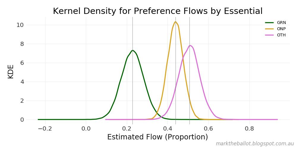
The results I got were very similar to the standard OLS results. In this case I have identified the 95% credible interval, which is the Bayesian equivalent of the confidence interval. Again, the One Nation and Other results are quite different, and swapped about between the two pollsters.
From Stan: for Essential
           2.5%    median     97.5%
GRN    0.121745  0.228054  0.335852
ONP    0.362631  0.438261  0.513884
OTH    0.404663  0.506283  0.607355
From Stan: for Newspoll
           2.5%    median     97.5%
GRN    0.089876  0.267659  0.450531
ONP    0.420720  0.494935  0.566663
OTH    0.259106  0.433838  0.601585
From the Bayesian analysis, our best guess is that Essential flows 23 per cent of the Green vote to the Coalition. It flows 44 per cent of the One Nation vote. And it flows 51 per cent of the Other vote. In comparison, Newspoll flows 27 per cent of the Green vote to the Coalition, 49 per cent of the One Nation vote, and 43 per cent of the Other vote.
These Bayesian results can be charted as probability densities as follows. In these charts the median sample for each distribution is highlighted with a thin vertical line.

For completeness, the supporting Python program that generated this analysis follows.
# PYTHON - estimates of preference flows from polling data

import pandas as pd
import numpy as np
import statsmodels.api as sm
import matplotlib.pyplot as plt

import sys
sys.path.append( '../bin' )
from stan_cache import stan_cache

# --- chart results
graph_dir = './Graphs/'
walk_leader = 'STAN-PREFERENCE-FLOWS-'
plt.style.use('../bin/markgraph.mplstyle')

# --- curate data for analysis
workbook = pd.ExcelFile('./Data/poll-data.xlsx')
df = workbook.parse('Data')

# drop polls without one nation
df = df[df['ONP'].notnull()]

# drop pre-2016 election data
df['MidDate'] = [pd.Period(d, freq='D') for d in df['MidDate']]
df = df[df['MidDate'] > pd.Period('2016-07-04', freq='D')]

# normalise the data - still in 0 to 100 range
parties = ['GRN', 'ONP', 'OTH']
all = ['L/NP', 'ALP'] + parties
df['Sum'] = df[all].sum(axis=1)
bad = df[all + ['Sum', 'Firm', 'Date']]
bad = bad[(bad['Sum'] < 99.5) | (bad['Sum'] > 100.5)]
print('--- Does not add to 100% ---')
print(bad)
print('----------------------------')
df[all] = df[all].div(df[all].sum(axis=1), axis=0) * 100.0

# --- Analyse the curated data
firms = df['Firm'].unique()
for firm in firms:
    cases = df[df['Firm']==firm]

    if len(cases) <= 10:
        continue # not enough to analyse

    # --- classic OLS multiple regression
    # get response vector and design matrix in 0 to 1 range
    y = (cases['TPP L/NP'] - cases['L/NP']) / 100.0
    X = cases[parties] / 100.0

    # regression estimation
    model = sm.OLS(y, X).fit()
    print('\n\n---- {} ----'.format(firm))
    # Print out the statistics
    print(model.summary())

    # --- let's do the same thing with Stan
    # input data
    data = {
        'y': y,
        'X' : X,
        'N': len(y),
        'k': len(X.columns)
    }

    # helpers
    quants = [2.5,  50, 97.5]
    labels = ['2.5%', 'median', '97.5%']

    with open ("./Models/preference flows.stan", "r") as file:
        model_code = file.read()
        file.close()

        # model
        stan = stan_cache(model_code=model_code, model_name='preference flows')
        fit = stan.sampling(data=data, iter=10000, chains=5)
        results = fit.extract()

        # capture the coefficients
        coefficients = results['beta']
        print('--- Coefficient Shape: {} ---'.format(coefficients.shape))
        estimates = pd.DataFrame()
        for i, party in zip(range(len(parties)), parties):
            q = np.percentile(coefficients[:,i], quants)
            row = pd.DataFrame(q, index=labels, columns=[party]).T
            estimates = estimates.append(row)

        # capture sigma
        sigma = results['sigma'].T
        q = np.percentile(sigma, quants)
        row = pd.DataFrame(q, index=labels, columns=['sigma']).T
        estimates = estimates.append(row)

        # print results from Stan
        print('From Stan: for {}'.format(firm))
        print(estimates)

        # plot results from Stan
        coefficients = pd.DataFrame(coefficients, columns=parties)
        ax = coefficients.plot.kde(color=['darkgreen', 'goldenrod', 'orchid'])
        ax.set_title('Kernel Density for Preference Flows by {}'.format(firm))
        ax.set_ylabel('KDE')
        ax.set_xlabel('Estimated Flow (Proportion)')
        for i in coefficients.columns:
            ax.axvline(x=coefficients[i].median(), color='gray', linewidth=0.5)

        fig = ax.figure
        fig.set_size_inches(8, 4)
        fig.tight_layout(pad=1)
        fig.text(0.99, 0.01, 'marktheballot.blogspot.com.au',
            ha='right', va='bottom', fontsize='x-small',
            fontstyle='italic', color='#999999')
        fig.savefig(graph_dir+walk_leader+firm+'.png', dpi=125)
        plt.close()
No comments:
Post a Comment