Redistributions

One of the myths of data science is the myth of scientific accuracy. The myth is that when a data scientist applies the correct mathematical procedures, they get a mathematical correct answer to seven decimal places. In reality, data scientists make many choices in the analysis they bring, and the data they work with. Gelman and Loken (2013) enlivened this concept to the statistics community with their paper on the garden of forking paths.

They way in which we curate data, munge it and prepare it for analysis, and the analytical frames we we use are all choices. Unconsciously those choices can frame our results. And they can blind us to the results we might have produced if we had taken a different approach. In short, they can mislead us, even when we set out to undertake ethical and unbiased analysis. 

I found myself reflecting on the garden of forking paths as I considered how to best apply the 2016 polling outcome data to the electoral boundary changes that occurred in 2017 and 2018. I wanted to find the best way to allocate to the new seat boundaries the ordinary votes that were geographically linked (via longitude and latitude) to polling locations in 2016 . I also had to allocate the non-tagged votes (some ordinary votes, but also absentee votes, provisional votes, postal votes and declaration pre-poll votes).

My initial plan was to allocate the 2016 two-party preferred (TPP) votes to new electorates based on the geo-coded place where the vote was cast. I would then allocate the remaining votes for each electorate in proportion with the geo-coded votes by party for that electorate. Once all the votes from 2016 had been allocated to the new electorate boundaries, I could calculate a TPP margin for each seat.

However, this turned out to be problematic. For example, a number of votes in the Victorian seat of Goldstein (which was unchanged by the Victorian redistribution) were coded as being cast outside of the electorate. But as the seat was unaffected by the redistribution, those votes should remain attributed to Goldstein, and should not be counted in another electorate.

The interesting analytical question became which data was most reflective of where people live (at a reasonably fine level of granularity), and which data is only reflective of the voter's electorate without any granularity about where in the electorate they might live. For example, if someone from the outer-suburbs of Melbourne votes in the city on polling day, can I draw any useful information about where they live in their electorate. My conclusion was that I could not.

As a consequence, to the extent I could apply this rule, where people voted at a polling booth outside of their electorate, and we have Geo-coding for that polling place, I chose to ignore that Geo-coding. I also decided to ignore the geo-coding for pre-poll votes. Because there are so few pre-poll voting centres, I assumed the votes cast at these centres were not necessarily informative about where in an electorate the pre-poll voters come from. Conversely, I assumed the location data from the many polling booths to be informative, if the person was casting an ordinary vote on the polling day in their electorate.

I was picky, because I wanted to be comfortable that as boundaries are redrawn, I was meaningfully attributing votes from the parts of an electorate that might be redistributed differently.

For the votes that I could only attribute to an electorate, I allocated them in the same proportion as the ordinary TPP votes by party were allocated. If 70 per cent of the Labor vote stayed in an electorate and 30 per cent went to another electorate, that is how I treated the Labor vote from the electorate where I did not have geographic information or where I deemed the geographic information I had to be insufficiently informative. I treated the flow of Coalition and Labor votes separately.

My initial results are close to, but also different from the work of others. My walk in the garden of forking paths was different to theirs. The usual caveats for preliminary analysis apply: Be warned, this work could include errors that I have not identified. While I have calculated results to two decimal places, this suggests a level of accuracy that belies the many choices I have made in munging and analysing the data. Also note: I could not find map data for the 2016 electorate boundaries in the shapefile format for NT and Tasmania, so my treatment of these states is less certain than the others.

And here are my Coalition 2016 TPP estimates for each seat compared with those from Antony Green and William Bowe.

Seat	Mark Graph	Antony Green	William Bowe
Bean (ACT)	40.9	41.1	41.1
Canberra (ACT)	36.54	36.8	36.8
Fenner (ACT)	38.97	38.4	38.2
Banks (NSW)	51.44	51.4	51.4
Barton (NSW)	41.7	41.7	41.7
Bennelong (NSW)	59.72	59.7	59.7
Berowra (NSW)	66.45	66.4	66.5
Blaxland (NSW)	30.52	30.5	30.5
Bradfield (NSW)	71.04	71	71
Calare (NSW)	61.81	61.8	61.8
Chifley (NSW)	30.81	30.8	30.8
Cook (NSW)	65.39	65.4	65.4
Cowper (NSW)	62.58	62.6	62.6
Cunningham (NSW)	36.68	36.7	36.7
Dobell (NSW)	45.19	45.2	45.2
Eden-Monaro (NSW)	47.07	47.1	47.1
Farrer (NSW)	70.53	70.5	70.5
Fowler (NSW)	32.51	32.5	32.5
Gilmore (NSW)	50.73	50.7	50.7
Grayndler (NSW)	27.64	27.6	27.6
Greenway (NSW)	43.69	43.7	43.7
Hughes (NSW)	59.33	59.3	59.3
Hume (NSW)	60.18	60.2	60.2
Hunter (NSW)	37.54	37.5	37.5
Kingsford Smith (NSW)	41.43	41.4	41.4
Lindsay (NSW)	48.89	48.9	48.9
Lyne (NSW)	61.63	61.6	61.6
Macarthur (NSW)	41.67	41.7	41.7
Mackellar (NSW)	65.74	65.7	65.7
Macquarie (NSW)	47.81	47.8	47.8
McMahon (NSW)	37.89	37.9	37.9
Mitchell (NSW)	67.82	67.8	67.8
New England (NSW)	66.42	66.4	66.4
Newcastle (NSW)	36.16	36.2	36.2
North Sydney (NSW)	63.61	63.6	63.6
Page (NSW)	52.3	52.3	52.3
Parkes (NSW)	65.1	65.1	65.1
Parramatta (NSW)	42.33	42.3	42.3
Paterson (NSW)	39.26	39.3	39.3
Reid (NSW)	54.69	54.7	54.7
Richmond (NSW)	46.04	46	46
Riverina (NSW)	66.44	66.4	66.4
Robertson (NSW)	51.14	51.1	51.1
Shortland (NSW)	40.06	40.1	40.1
Sydney (NSW)	34.69	34.7	34.7
Warringah (NSW)	61.09	61.1	61.1
Watson (NSW)	32.42	32.4	32.4
Wentworth (NSW)	67.75	67.7	67.8
Werriwa (NSW)	41.8	41.8	41.8
Whitlam (NSW)	36.28	36.3	36.3
Lingiari (NT)	41.58	41.9	41.8
Solomon (NT)	44	43.9	43.9
Blair (Qld)	41.81	42	41.8
Bonner (Qld)	53.39	53.4	53.4
Bowman (Qld)	57.07	57.1	57.1
Brisbane (Qld)	55.85	56	56.1
Capricornia (Qld)	50.63	50.6	50.6
Dawson (Qld)	53.37	53.3	53.4
Dickson (Qld)	51.6	52	52
Fadden (Qld)	61.05	61.2	61.3
Fairfax (Qld)	60.78	61	60.8
Fisher (Qld)	59.24	59.2	59.3
Flynn (Qld)	51.04	51	51
Forde (Qld)	50.63	50.6	50.6
Griffith (Qld)	48.93	48.6	48.7
Groom (Qld)	65.31	65.3	65.3
Herbert (Qld)	49.98	49.98	50
Hinkler (Qld)	58.42	58.4	58.4
Kennedy (Qld)
Leichhardt (Qld)	53.89	54	53.9
Lilley (Qld)	44.68	44.2	44.2
Longman (Qld)	49.21	49.2	49.2
Maranoa (Qld)	67.54	67.5	67.5
McPherson (Qld)	61.64	61.6	61.6
Moncrieff (Qld)	64.94	64.5	64.7
Moreton (Qld)	45.58	46	45.9
Oxley (Qld)	40.92	40.9	40.9
Petrie (Qld)	51.65	51.6	51.7
Rankin (Qld)	38.7	38.7	38.7
Ryan (Qld)	59.21	58.8	59.1
Wide Bay (Qld)	58.14	58.3	58.2
Wright (Qld)	59.62	59.6	59.6
Adelaide (SA)	40.5	41	41.1
Barker (SA)	64.13	64.3	64.1
Boothby (SA)	52.74	52.8	52.9
Grey (SA)	58.37	58.5	58.1
Hindmarsh (SA)	42.64	41.8	41.8
Kingston (SA)	36.21	36.5	36.4
Makin (SA)	39.04	39.1	39.2
Mayo (SA)
Spence (SA)	31.79	32.1	32.2
Sturt (SA)	55.78	55.8	55.7
Bass (Tas)	44.57	44.7	44.5
Braddon (Tas)	48.43	48.5	48.4
Clark (Tas)
Franklin (Tas)	39.3	39.3	39.3
Lyons (Tas)	46.12	46	46.9
Aston (Vic)	57.73	57.6	57.4
Ballarat (Vic)	42.55	42.6	42.6
Bendigo (Vic)	45.98	46.1	46.1
Bruce (Vic)	33.5	34.3	34.5
Calwell (Vic)	27.88	29.9	29.7
Casey (Vic)	54.03	54.5	54.3
Chisholm (Vic)	53.54	53.4	53.4
Cooper (Vic)	28.25	28	27.9
Corangamite (Vic)	50.61	50.03	50
Corio (Vic)	40.84	41.7	41.5
Deakin (Vic)	56.11	56.3	56.6
Dunkley (Vic)	48.79	48.7	48.7
Flinders (Vic)	56.64	57.2	57.1
Fraser (Vic)	29.85	29.4	29.5
Gellibrand (Vic)	35.68	35.3	35.3
Gippsland (Vic)	68.13	68.2	68.1
Goldstein (Vic)	62.68	62.7	62.7
Gorton (Vic)	32.59	31.7	31.7
Higgins (Vic)	60.64	60.2	60.3
Holt (Vic)	40.16	40.1	40.2
Hotham (Vic)	44.89	45.8	45.8
Indi (Vic)
Isaacs (Vic)	48.69	47.7	47.8
Jagajaga (Vic)	46.03	45	45
Kooyong (Vic)	63.14	62.8	62.9
La Trobe (Vic)	52.68	53.5	52.4
Lalor (Vic)	34.6	35.6	35.6
Macnamara (Vic)	48.41	48.7	48.6
Mallee (Vic)	69.42	69.8	69.6
Maribyrnong (Vic)	40.18	40.6	40.6
McEwen (Vic)	44.03	44.7	44.6
Melbourne (Vic)
Menzies (Vic)	58.2	57.9	57.9
Monash (Vic)	58.02	57.6	57.8
Nicholls (Vic)	72.49	72.3	72.4
Scullin (Vic)	27.26	29.6	29.7
Wannon (Vic)	59.59	59.3	59.3
Wills (Vic)	28.07	28.2	28.3
Brand (WA)	38.57	38.6	38.6
Burt (WA)	42.89	42.9	42.9
Canning (WA)	56.79	56.8	56.8
Cowan (WA)	49.32	49.3	49.3
Curtin (WA)	70.7	70.7	70.7
Durack (WA)	61.06	61.1	61.1
Forrest (WA)	62.56	62.6	62.6
Fremantle (WA)	42.48	42.5	42.5
Hasluck (WA)	52.05	52.1	52.1
Moore (WA)	61.02	61	61
O'Connor (WA)	65.04	65	65
Pearce (WA)	53.63	53.6	53.6
Perth (WA)	46.67	46.7	46.7
Stirling (WA)	56.12	56.1	56.1
Swan (WA)	53.59	53.6	53.6
Tangney (WA)	61.07	61.1	61.1

Archive from 2016 Australian Federal Election

Note: the following page is the approach I took to the 2016 Federal Election. The Bayesian Aggregation page is being/has been updated for the 2019 election ...

This page provides some technical background on the Bayesian poll aggregation models used on this site. The page has been updated for the 2016 Federal election.

General overview

The aggregation or data fusion models I use are known as hidden Markov models. They are are sometimes referred to as state space models or latent process models.

I model the national voting intention (which cannot be observed directly; it is "hidden") for each and every day of the period under analysis. The only time the national voting intention is not hidden, is at an election. In some models (known as anchored models), we use the election result to anchor the daily model we use.

In the language of modelling, our estimates of the national voting intention for each day being modeled are known as states. These "states" link together to form a Markov process, where each state is directly dependent on the previous state and a probability distribution linking the states. In plain English, the models assume that the national voting intention today is much like it was yesterday. The simplest models assume the voting intention today is normally distributed around the voting intention yesterday.

The model is informed by irregular and noisy data from the selected polling houses. The challenge for the model is to ignore the noise and find the underlying signal. In effect, the model is solved by finding the the day-to-day pathway with the maximum likelihood given the known poll results.

To improve the robustness of the model, we make provision for the long-run tendency of each polling house to systematically favour either the Coalition or Labor. We call this small tendency to favour one side or the other a "house effect". The model assumes that the results from each pollster diverge (on average) from the from real population voting intention by a small, constant number of percentage points. We use the calculated house effect to adjust the raw polling data from each polling house.

In estimating the house effects, we can take one of a number of approaches. We could:

• anchor the model to an election result on a particular day, and use that anchoring to establish the house effects.
• anchor the model to a particular polling house or houses; or 
• assume that collectively the polling houses are unbiased, and that collectively their house effects sum to zero.

Typically, I use the first and third approaches in my models. Some models assume that the house effects sum to zero. Other models assume that the house effects can be determined absolutely by anchoring the hidden model for a particular day or week to a known election outcome.

There are issues with both approaches. The problem with anchoring the model to an election outcome (or to a particular polling house), is that pollsters are constantly reviewing and, from time to time, changing their polling practice. Over time these changes affect the reliability of the model. On the other hand, the sum-to-zero assumption is rarely correct. Of the two approaches, anchoring tends to perform better.

Another adjustment we make is to allow discontinuities in the hidden process when either party changes its leadership. Leadership changes can see immediate changes in the voting preferences. For the anchored models, we allow for discontinuities with the Gillard to Rudd and Abbott to Turnbull leadership changes. The unanchored models have a single discontinuity with the Abbott to Turnbull leadership change.

Solving a model necessitates integration over a series of complex multidimensional probability distributions. The definite integral is typically impossible to solve algebraically. But it can be solved using a numerical method based on Markov chains and random numbers known as Markov Chain Monte Carlo (MCMC) integration. I use a free software product called JAGS to solve these models.

The dynamic linear model of TPP voting intention with house effects summed to zero

This is the simplest model. It has three parts:

1. The observational part of the model assumes two factors explain the difference between published poll results (what we observe) and the national voting intention on a particular day (which, with the exception of elections, is hidden):
   
   
   1. The first factor is the margin of error from classical statistics. This is the random error associated with selecting a sample; and
   2. The second factor is the systemic biases (house effects) that affect each pollster's published estimate of the population voting intention.
   
   
2. The temporal part of the model assumes that the actual population voting intention on any day is much the same as it was on the previous day (with the exception of discontinuities). The model estimates the (hidden) population voting intention for every day under analysis.


3. The house effects part of the model assumes that house effects are distributed around zero and sum to zero.

This model builds on original work by Professor Simon Jackman. It is encoded in JAGS as follows:

model {
    ## -- draws on models developed by Simon Jackman

    ## -- observational model
    for(poll in 1:n_polls) { 
        yhat[poll] <- houseEffect[house[poll]] + hidden_voting_intention[day[poll]]
        y[poll] ~ dnorm(yhat[poll], samplePrecision[poll]) # distribution
    }

    ## -- temporal model - with one discontinuity
    hidden_voting_intention[1] ~ dunif(0.3, 0.7) # contextually uninformative
    hidden_voting_intention[discontinuity] ~ dunif(0.3, 0.7) # ditto
    
    for(i in 2:(discontinuity-1)) { 
        hidden_voting_intention[i] ~ dnorm(hidden_voting_intention[i-1], walkPrecision)
    }
    for (j in (discontinuity+1):n_span) {
        hidden_voting_intention[j] ~ dnorm(hidden_voting_intention[j-1], walkPrecision)
    }
    sigmaWalk ~ dunif(0, 0.01)
    walkPrecision <- pow(sigmaWalk, -2)

    ## -- house effects model
    for(i in 2:n_houses) { 
        houseEffect[i] ~ dunif(-0.15, 0.15) # contextually uninformative
    }
    houseEffect[1] <- -sum( houseEffect[2:n_houses] )
}

Professor Jackman's original JAGS code can be found in the file kalman.bug, in the zip file link on this page, under the heading Pooling the Polls Over an Election Campaign.

The anchored dynamic linear model of TPP voting intention

This model is much the same as the previous model. However, it is run with data from prior to the 2013 election to anchor poll performance. It includes two discontinuities, with the ascensions of Rudd and Turnbull. And, because it is anchored, the house effects are not constrained to sum to zero.

model {

    ## -- observational model
    for(poll in 1:n_polls) { 
        yhat[poll] <- houseEffect[house[poll]] + hidden_voting_intention[day[poll]]
        y[poll] ~ dnorm(yhat[poll], samplePrecision[poll]) # distribution
    }


    ## -- temporal model - with two or more discontinuities 
    # priors ...
    hidden_voting_intention[1] ~ dunif(0.3, 0.7) # fairly uninformative
    for(j in 1:n_discontinuities) {
        hidden_voting_intention[discontinuities[j]] ~ dunif(0.3, 0.7) # fairly uninformative
    }
    sigmaWalk ~ dunif(0, 0.01)
    walkPrecision <- pow(sigmaWalk, -2)
    
    # Up until the first discontinuity ...  
    for(k in 2:(discontinuities[1]-1)) {
        hidden_voting_intention[k] ~ dnorm(hidden_voting_intention[k-1], walkPrecision)   
    }
    
    # Between the discontinuities ... assumes 2 or more discontinuities ...
    for( disc in 1:(n_discontinuities-1) ) {
        for(k in (discontinuities[disc]+1):(discontinuities[(disc+1)]-1)) {
            hidden_voting_intention[k] ~ dnorm(hidden_voting_intention[k-1], walkPrecision)   
        }
    }    
    
    # after the last discontinuity
    for(k in (discontinuities[n_discontinuities]+1):n_span) {
        hidden_voting_intention[k] ~ dnorm(hidden_voting_intention[k-1], walkPrecision)   
    }


    ## -- house effects model
    for(i in 1:n_houses) { 
        houseEffect[i] ~ dnorm(0, pow(0.05, -2))
    }
}

The latent Dirichlet process for primary voting intention

This model is more complex. It takes advantage of the Dirichlet (pronounced dirik-lay) distribution, which always sums to 1, just as the primary votes for all parties would sum to 100 per cent of voters at an election. A weakness is a transmission mechanism from day-to-day that uses a "tightness of fit" parameter, which has been arbitrarily selected.

The model is set up a little differently to the previous models. Rather than pass the vote share as a number between 0 and 1; we pass the size of the sample that indicated a preference for each party. For example, if the poll is of 1000 voters, with 40 per cent for the Coalition, 40 per cent for Labor, 11 per cent for the Greens and and 9 per cent for Other parties, the multinomial we would pass across for this poll is [400, 400, 110, 90]. 

More broadly, this model is conceptually very similar to the sum-to-zero TPP model: with an observational component, a dynamic walk of primary voting proportions (modeled as a hierarchical Dirichlet process), a discontinuity for Turnbull's ascension, and a set of house effects that sum to zero across polling houses and across the parties.

data {
    zero <- 0.0
}
model {

    #### -- observational model
    
    for(poll in 1:NUMPOLLS) { # for each poll result - rows
        adjusted_poll[poll, 1:PARTIES] <- walk[pollDay[poll], 1:PARTIES] +
            houseEffect[house[poll], 1:PARTIES]
        primaryVotes[poll, 1:PARTIES] ~ dmulti(adjusted_poll[poll, 1:PARTIES], n[poll])
    }


    #### -- temporal model with one discontinuity
    
    tightness <- 50000 # kludge - today very much like yesterday
    # - before discontinuity
    for(day in 2:(discontinuity-1)) { 
        # Note: use math not a distribution to generate the multinomial ...
        multinomial[day, 1:PARTIES] <- walk[day-1,  1:PARTIES] * tightness
        walk[day, 1:PARTIES] ~ ddirch(multinomial[day, 1:PARTIES])
    }
    # - after discontinuity
    for(day in discontinuity+1:PERIOD) { 
        # Note: use math not a distribution to generate the multinomial ...
        multinomial[day, 1:PARTIES] <- walk[day-1,  1:PARTIES] * tightness
        walk[day, 1:PARTIES] ~ ddirch(multinomial[day, 1:PARTIES])
    }

    ## -- weakly informative priors for first and discontinuity days
    for (party in 1:2) { # for each major party
        alpha[party] ~ dunif(250, 600) # majors between 25% and 60%
        beta[party] ~ dunif(250, 600) # majors between 25% and 60%
    }
    for (party in 3:PARTIES) { # for each minor party
        alpha[party] ~ dunif(10, 250) # minors between 1% and 25%
        beta[party] ~ dunif(10, 250) # minors between 1% and 25%
    }
    walk[1, 1:PARTIES] ~ ddirch(alpha[])
    walk[discontinuity, 1:PARTIES] ~ ddirch(beta[])

    ## -- estimate a Coalition TPP from the primary votes
    for(day in 1:PERIOD) {
        CoalitionTPP[day] <- sum(walk[day, 1:PARTIES] *
            preference_flows[1:PARTIES])
        CoalitionTPP2010[day] <- sum(walk[day, 1:PARTIES] *
            preference_flows_2010[1:PARTIES])
    }


    #### -- house effects model with two-way, sum-to-zero constraints

    ## -- vague priors ...
    for (h in 2:HOUSECOUNT) { 
        for (p in 2:PARTIES) { 
            houseEffect[h, p] ~ dunif(-0.1, 0.1)
       }
    }

    ## -- sum to zero - but only in one direction for houseEffect[1, 1]
    for (p in 2:PARTIES) { 
        houseEffect[1, p] <- 0 - sum( houseEffect[2:HOUSECOUNT, p] )
    }
    for(h in 1:HOUSECOUNT) { 
        # includes constraint for houseEffect[1, 1], but only in one direction
        houseEffect[h, 1] <- 0 - sum( houseEffect[h, 2:PARTIES] )
    }

    ## -- the other direction constraint on houseEffect[1, 1]
    zero ~ dsum( houseEffect[1, 1], sum( houseEffect[2:HOUSECOUNT, 1] ) )
}

The anchored Dirichlet primary vote model

The anchored Dirichlet model follows. It draws on elements from the anchored TPP model and Dirichlet model above. It is the most complex of these models. It also takes the longest time to produce reliable results. For this model, I run 460,000 samples, taking every 23rd sample for analysis. On my aging Apple iMac and JAGS 4.0.1 it takes around 100 minutes to run. 

model {

    #### -- observational model
    for(poll in 1:NUMPOLLS) { # for each poll result - rows
        adjusted_poll[poll, 1:PARTIES] <- walk[pollDay[poll], 1:PARTIES] +
            houseEffect[house[poll], 1:PARTIES]
        primaryVotes[poll, 1:PARTIES] ~ dmulti(adjusted_poll[poll, 1:PARTIES], n[poll])
    }

    #### -- temporal model with multiple discontinuities
    # - tightness of fit parameters
    tightness <- 50000 # kludge - today very much like yesterday    
    
    # Up until the first discontinuity ...  
    for(day in 2:(discontinuities[1]-1)) {
        multinomial[day, 1:PARTIES] <- walk[day-1,  1:PARTIES] * tightness
        walk[day, 1:PARTIES] ~ ddirch(multinomial[day, 1:PARTIES])
    }
    
    # Between the discontinuities ... assumes 2 or more discontinuities ...
    for( disc in 1:(n_discontinuities-1) ) {
        for(day in (discontinuities[disc]+1):(discontinuities[(disc+1)]-1)) {
            multinomial[day, 1:PARTIES] <- walk[day-1,  1:PARTIES] * tightness
            walk[day, 1:PARTIES] ~ ddirch(multinomial[day, 1:PARTIES])
        }
    }    
    
    # After the last discontinuity
    for(day in (discontinuities[n_discontinuities]+1):PERIOD) {
        multinomial[day, 1:PARTIES] <- walk[day-1,  1:PARTIES] * tightness
        walk[day, 1:PARTIES] ~ ddirch(multinomial[day, 1:PARTIES])
    }

    # weakly informative priors for first day and discontinutity days ...
    for (party in 1:2) { # for each minor party
        alpha[party] ~ dunif(250, 600) # minors between 25% and 60%
    }
    for (party in 3:PARTIES) { # for each minor party
        alpha[party] ~ dunif(10, 200) # minors between 1% and 20%
    }
    walk[1, 1:PARTIES] ~ ddirch(alpha[])
    
    for(j in 1:n_discontinuities) {
        for (party in 1:2) { # for each minor party
            beta[j, party] ~ dunif(250, 600) # minors between 25% and 60%
        }
        for (party in 3:PARTIES) { # for each minor party
            beta[j, party] ~ dunif(10, 200) # minors between 1% and 20%
        }
        walk[discontinuities[j], 1:PARTIES] ~ ddirch(beta[j, 1:PARTIES])
    }

    ## -- estimate a Coalition TPP from the primary votes
    for(day in 1:PERIOD) {
        CoalitionTPP[day] <- sum(walk[day, 1:PARTIES] *
            preference_flows[1:PARTIES])
    }

    #### -- sum-to-zero constraints on house effects
    for(h in 1:HOUSECOUNT) { 
        for (p in 2:PARTIES) { 
            houseEffect[h, p] ~ dnorm(0, pow(0.05, -2))
       }
    }
    # need to lock in ... but only in one dimension
    for(h in 1:HOUSECOUNT) { # for each house ...
        houseEffect[h, 1] <- -sum( houseEffect[h, 2:PARTIES] )
    }
}

Beta model of primary vote share for Palmer United

A simplification of the Dirichlet distribution is the Beta distribution. I use the Beta distribution (in a similar model to the Dirichlet model above), to track the primary vote share of the Palmer United Party. This model does not provide for a discontinuity in voting associated with the change of Prime Minister.

model {

    #### -- observational model
    for(poll in 1:NUMPOLLS) { # for each poll result - rows
        adjusted_poll[poll] <- walk[pollDay[poll]] + houseEffect[house[poll]]
        palmerVotes[poll] ~ dbin(adjusted_poll[poll], n[poll])
    }

    #### -- temporal model (a daily walk where today is much like yesterday)
    tightness <- 50000 # KLUDGE - tightness of fit parameter selected by hand
    for(day in 2:PERIOD) { # rows
        binomial[day] <- walk[day-1] * tightness
        walk[day] ~ dbeta(binomial[day], tightness - binomial[day])
    }

    ## -- weakly informative priors for first day in the temporal model
    alpha ~ dunif(1, 1500)
    walk[1] ~ dbeta(alpha, 10000-alpha)

    #### -- sum-to-zero constraints on house effects
    for(h in 2:HOUSECOUNT) { # for each house ...
        houseEffect[h] ~ dnorm(0, pow(0.1, -2))
    }
    houseEffect[1] <- -sum(houseEffect[2:HOUSECOUNT])
}

Code and data

I have made most of my data and code base available on Google Drive. Please note, this is my live code base, which I play with quite a bit. So, there will be times when it is broken or in some stage of being edited.

What I have not made available is the Excel spreadsheets into which I initially place my data. These live in the (hidden) raw-data directory. However, the collated data for the Bayesian model lives in the intermediate directory, visible from the above link.

Australian Federal Voting Practice

Today's charts take a quick look at the number and proportion of formal votes cast at recent Federal elections by vote type in the House of Representatives. Before each chart is a quick definition of the vote type.

An Absent Vote is cast on election day, but at a polling place outside of the voter's electorate, but still within the state or territory.

An Ordinary Vote is cast on election day at a polling place within the electoral division for which a voter is enrolled.

A Postal Vote is cast by post because the voter cannot attend a polling place in their state or territory on election day.

A Pre-poll Vote is cast at an early voting centre or an AEC divisional office before election day.

A Provisional Vote is one cast when a voter's name cannot be found on the certified list, the voter's name is already marked off the certified list as having voted, or the voter is registered as a silent elector.

Yielding a total formal vote count as follows.

A Formal Vote is cast when the ballot paper has been marked according to the rules for that election and can be counted towards the result. A ballot paper that does not meet the rules for formality is called informal and cannot be counted towards the result.

Confessions of a failed forecaster

Let's be frank: I had a shocking election. My aggregated forecast of 51.4 per cent for the Coalition in two-party preferred (TPP) terms was off, way off. The final outcome was a good percentage point lower at 50.35 per cent. 

My error was simple. I had assumed that the pollster biases from the 2013 election would be much the same in 2016. Ironically, I was alerted to the error of my ways shortly before the election when Nate Silver blogged in early June 2016, 

The good news is that, over the long run, the polls haven’t had much of an overall bias, having underrated Republicans in some elections and Democrats in others. But the bias has shifted around somewhat unpredictably from election to election. You should be wary of claims that the polls are bound to be biased in the same direction that they were two years ago or four years ago.

Although I run both 2013-biased and unbiased models, I doubled down on the middle ranked biased model without testing the robustness of my assumptions. To add insult to injury, my unbiased models came in much closer to the final result. The unbiased TPP model projected the Coalition would get 50.6 per cent of the TPP vote share. The unbiased primary vote model projected 50.5 per cent.

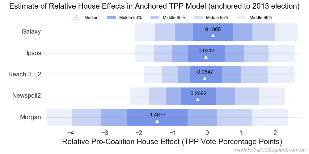
Now that I have got that off my chest, let's have a closer look at the path of the polls over the election period and evaluate the performance of the pollsters. If we anchor a daily walk of the TPP estimate from aggregating the polls to the election outcome, we get the following.

My results suggest that Ipsos was the most accurate pollster over the election period. But to be fair, There was only a whisker in it between Ipsos, Galaxy, ReachTEL and Newspoll.

These results also suggest that Turnbull snatched outright victory (albeit a slim one) from what looked like a hung parliament early in the longer-than-usual election period. The cloud of poll results in the last quarter of this period were the most favourable to Turnbull.

If we focus on the primary votes, the story becomes a little more nuanced. Over the course of the election period the majors - but particularly Labor - lost primary vote share to the Others. This movement from Labor to Others may have been behind the Coalition's whisper thin win in the end.

While the Greens improved on their 2013 result (from 8.65 to 10.23 per cent of the primary vote share), they under-performed against their pre-election polling. The Green's primary vote trajectory was downwards for most of the period

The Coalition did worse than 2013 with preference flows. If they had achieved the same preference flows in 2016 as 2013, they would have achieved a TPP vote share of 50.6 per cent. This is significant: Up until the 2016 election, it was possible that the historically low preference flows in 2013 where anomalous.

My suspicion is that we are seeing fracturing of he left in Australian politics, where more and more people who do not want to vote Coalition, also feel uncomfortable with Labor in the first instance (even though in most cases the preference from those voters ultimately flows to Labor).

Well that is enough confession for this Sunday. Over the coming months I will look at other aspects of the 2016 election in more detail. As polls this far out from an election are of little predictive value, I will take a holiday from poll aggregation for the next 12 to 18 months or so.

Monte Carlo Simulation of Poll Results

I have brought together some disparate data so that I can use Monte Carlo techniques to simulate an election outcome (1,000,000 times) from yesterday's poll aggregation result (51.6 per cent in the Coalition's favour).

The first step was to establish the state and national starting points (ie. the TPP results from the 2013 election). For this data, I went to the AEC: http://results.aec.gov.au/17496/Website/HouseTppByState-17496.htm.

The national swing is the latest poll aggregation minus the 2013 TPP result. A negative result means a swing to Labor. A positive result is a swing to the Coalition.

To establish the relative swings in each state, I used the latest Newspoll results for June in today's Australian and compared them with the Newspoll national swing since the 2013 election. The relative swings (in percentage points) I calculated were as follows. These are added to the national swing. A negative relative swing moves a state more to Labor than the national swing. A positive swing moves a state less to Labor than the national swing.

	NSW	VIC	QLD	WA	SA	TAS	ACT	NT
0	-0.1	1.7	-2.5	-0.8	2.5	0	0	0

These swings were applied to the pendulum from the 2013 election, as adjusted for the new electoral boundaries. I used Antony Green's pendulum. The results were converted into a probability of a Coalition or Labor victory. The conversion used a cumulative density function from scipy.stats, with a standard deviation of 2.7 percentage points.

This approach did not work for all seats. It did not work for seats where an independent had won in 2013. Nor did it work for seats where independents, the Greens or Xenophon might win in 2016. For the following set of seats I substituted the poll derived probability with a betting market probability, adjusted for the longshot bias: Melbourne (VIC), Denison (TAS), Indi (VIC), Kennedy (QLD), Fairfax (QLD), Cowper (NSW), New England (NSW), Barker (SA), Boothby (SA), Grey (SA), Mayo (SA) and Batman (VIC).

From here I applied a Monte Carlo simulation for 1,000,000 iterations. With the usual caveats that go with code that has been slapped together in an hour and a half (ie. these results could be completely bogus and riddled with human error), the results of the simulation were as follows. The most likely seat outcome is 79 seats for the Coalition, 65 for Labor, and 6 others. The Coalition has an 87.7 per cent chance of forming majority government.

The seat probabilities I used for this Monte Carlo simulation are as follows.

	Any Other	Coalition	Green	Ind	Katter	Labor	NXT
Seat
Mallee (VIC)	0	1.000000e+00	0.000000	0.000000	0	0.000000e+00	0.000000
Maranoa (QLD)	0	1.000000e+00	0.000000	0.000000	0	1.812495e-11	0.000000
Farrer (NSW)	0	1.000000e+00	0.000000	0.000000	0	1.217915e-13	0.000000
Mitchell (NSW)	0	1.000000e+00	0.000000	0.000000	0	3.635980e-13	0.000000
Bradfield (NSW)	0	1.000000e+00	0.000000	0.000000	0	1.384115e-12	0.000000
Murray (VIC)	0	1.000000e+00	0.000000	0.000000	0	9.658940e-15	0.000000
Parkes (NSW)	0	1.000000e+00	0.000000	0.000000	0	1.812495e-11	0.000000
Berowra (NSW)	0	1.000000e+00	0.000000	0.000000	0	1.635948e-10	0.000000
Riverina (NSW)	0	1.000000e+00	0.000000	0.000000	0	1.635948e-10	0.000000
Wentworth (NSW)	0	1.000000e+00	0.000000	0.000000	0	2.075012e-10	0.000000
Mackellar (NSW)	0	1.000000e+00	0.000000	0.000000	0	2.628390e-10	0.000000
Curtin (WA)	0	1.000000e+00	0.000000	0.000000	0	5.028657e-09	0.000000
Moncrieff (QLD)	0	9.999997e-01	0.000000	0.000000	0	2.503352e-07	0.000000
Groom (QLD)	0	9.999961e-01	0.000000	0.000000	0	3.901843e-06	0.000000
Cook (NSW)	0	9.999998e-01	0.000000	0.000000	0	1.697103e-07	0.000000
Gippsland (VIC)	0	1.000000e+00	0.000000	0.000000	0	4.039625e-09	0.000000
North Sydney (NSW)	0	9.999998e-01	0.000000	0.000000	0	2.062545e-07	0.000000
O'Connor (WA)	0	9.999984e-01	0.000000	0.000000	0	1.614523e-06	0.000000
Warringah (NSW)	0	9.999996e-01	0.000000	0.000000	0	4.440377e-07	0.000000
Durack (WA)	0	9.999981e-01	0.000000	0.000000	0	1.931239e-06	0.000000
Calare (NSW)	0	9.999992e-01	0.000000	0.000000	0	7.782812e-07	0.000000
Menzies (VIC)	0	9.999999e-01	0.000000	0.000000	0	6.274431e-08	0.000000
Fadden (QLD)	0	9.998891e-01	0.000000	0.000000	0	1.109331e-04	0.000000
Forrest (WA)	0	9.999850e-01	0.000000	0.000000	0	1.495149e-05	0.000000
Hume (NSW)	0	9.999909e-01	0.000000	0.000000	0	9.124021e-06	0.000000
Lyne (NSW)	0	9.999909e-01	0.000000	0.000000	0	9.124021e-06	0.000000
Wide Bay (QLD)	0	9.994195e-01	0.000000	0.000000	0	5.805289e-04	0.000000
McPherson (QLD)	0	9.992488e-01	0.000000	0.000000	0	7.512405e-04	0.000000
Tangney (WA)	0	9.999288e-01	0.000000	0.000000	0	7.123697e-05	0.000000
Moore (WA)	0	9.998293e-01	0.000000	0.000000	0	1.707408e-04	0.000000
Flinders (VIC)	0	9.999909e-01	0.000000	0.000000	0	9.124021e-06	0.000000
Hughes (NSW)	0	9.998519e-01	0.000000	0.000000	0	1.480729e-04	0.000000
McMillan (VIC)	0	9.999909e-01	0.000000	0.000000	0	9.124021e-06	0.000000
Wright (QLD)	0	9.968310e-01	0.000000	0.000000	0	3.169028e-03	0.000000
Canning (WA)	0	9.992488e-01	0.000000	0.000000	0	7.512405e-04	0.000000
Kooyong (VIC)	0	9.999716e-01	0.000000	0.000000	0	2.836012e-05	0.000000
Goldstein (VIC)	0	9.999668e-01	0.000000	0.000000	0	3.317359e-05	0.000000
Sturt (SA)	0	9.999612e-01	0.000000	0.000000	0	3.875334e-05	0.000000
Wannon (VIC)	0	9.998718e-01	0.000000	0.000000	0	1.282479e-04	0.000000
Higgins (VIC)	0	9.998293e-01	0.000000	0.000000	0	1.707408e-04	0.000000
Fisher (QLD)	0	9.766504e-01	0.000000	0.000000	0	2.334957e-02	0.000000
Pearce (WA)	0	9.925224e-01	0.000000	0.000000	0	7.477578e-03	0.000000
Hinkler (QLD)	0	9.547458e-01	0.000000	0.000000	0	4.525416e-02	0.000000
Stirling (WA)	0	9.898930e-01	0.000000	0.000000	0	1.010699e-02	0.000000
Bowman (QLD)	0	9.511072e-01	0.000000	0.000000	0	4.889277e-02	0.000000
Ryan (QLD)	0	9.341635e-01	0.000000	0.000000	0	6.583650e-02	0.000000
Aston (VIC)	0	9.984213e-01	0.000000	0.000000	0	1.578708e-03	0.000000
Bennelong (NSW)	0	9.837078e-01	0.000000	0.000000	0	1.629221e-02	0.000000
Dawson (QLD)	0	8.798433e-01	0.000000	0.000000	0	1.201567e-01	0.000000
Swan (WA)	0	9.547458e-01	0.000000	0.000000	0	4.525416e-02	0.000000
Casey (VIC)	0	9.950830e-01	0.000000	0.000000	0	4.917013e-03	0.000000
Longman (QLD)	0	8.198897e-01	0.000000	0.000000	0	1.801103e-01	0.000000
Dickson (QLD)	0	7.997898e-01	0.000000	0.000000	0	2.002102e-01	0.000000
Flynn (QLD)	0	7.783987e-01	0.000000	0.000000	0	2.216013e-01	0.000000
Herbert (QLD)	0	7.439867e-01	0.000000	0.000000	0	2.560133e-01	0.000000
Burt (WA)	0	8.940354e-01	0.000000	0.000000	0	1.059646e-01	0.000000
Hasluck (WA)	0	8.870985e-01	0.000000	0.000000	0	1.129015e-01	0.000000
Leichhardt (QLD)	0	6.810012e-01	0.000000	0.000000	0	3.189988e-01	0.000000
Dunkley (VIC)	0	9.766504e-01	0.000000	0.000000	0	2.334957e-02	0.000000
Cowan (WA)	0	7.439867e-01	0.000000	0.000000	0	2.560133e-01	0.000000
Macquarie (NSW)	0	8.198897e-01	0.000000	0.000000	0	1.801103e-01	0.000000
Forde (QLD)	0	4.956192e-01	0.000000	0.000000	0	5.043808e-01	0.000000
Brisbane (QLD)	0	4.808508e-01	0.000000	0.000000	0	5.191492e-01	0.000000
Bass (TAS)	0	7.783987e-01	0.000000	0.000000	0	2.216013e-01	0.000000
La Trobe (Vic)	0	9.187069e-01	0.000000	0.000000	0	8.129310e-02	0.000000
Corangamite (VIC)	0	9.129883e-01	0.000000	0.000000	0	8.701166e-02	0.000000
Gilmore (NSW)	0	7.439867e-01	0.000000	0.000000	0	2.560133e-01	0.000000
Bonner (QLD)	0	3.934876e-01	0.000000	0.000000	0	6.065124e-01	0.000000
Reid (NSW)	0	6.941110e-01	0.000000	0.000000	0	3.058890e-01	0.000000
Macarthur (NSW)	0	6.810012e-01	0.000000	0.000000	0	3.189988e-01	0.000000
Deakin (VIC)	0	8.643622e-01	0.000000	0.000000	0	1.356378e-01	0.000000
Page (NSW)	0	6.541047e-01	0.000000	0.000000	0	3.458953e-01	0.000000
Robertson (NSW)	0	6.541047e-01	0.000000	0.000000	0	3.458953e-01	0.000000
Lindsay (NSW)	0	6.403480e-01	0.000000	0.000000	0	3.596520e-01	0.000000
Eden Monaro (NSW)	0	6.264070e-01	0.000000	0.000000	0	3.735930e-01	0.000000
Banks (NSW)	0	5.836504e-01	0.000000	0.000000	0	4.163496e-01	0.000000
Braddon (TAS)	0	5.980403e-01	0.000000	0.000000	0	4.019597e-01	0.000000
Hindmarsh (SA)	0	8.198897e-01	0.000000	0.000000	0	1.801103e-01	0.000000
Solomon (NT)	0	4.222399e-01	0.000000	0.000000	0	5.777601e-01	0.000000
Lyons (TAS)	0	3.934876e-01	0.000000	0.000000	0	6.065124e-01	0.000000
Capricornia (QLD)	0	8.942334e-02	0.000000	0.000000	0	9.105767e-01	0.000000
Petrie (QLD)	0	7.277572e-02	0.000000	0.000000	0	9.272243e-01	0.000000
Dobell (NSW)	0	2.044599e-01	0.000000	0.000000	0	7.955401e-01	0.000000
McEwen (VIC)	0	4.367835e-01	0.000000	0.000000	0	5.632165e-01	0.000000
Paterson (NSW)	0	1.840947e-01	0.000000	0.000000	0	8.159053e-01	0.000000
Lingiari (NT)	0	1.473151e-01	0.000000	0.000000	0	8.526849e-01	0.000000
Bendigo (VIC)	0	2.855145e-01	0.000000	0.000000	0	7.144855e-01	0.000000
Lilley (QLD)	0	1.691499e-02	0.000000	0.000000	0	9.830850e-01	0.000000
Parramatta (NSW)	0	1.087499e-01	0.000000	0.000000	0	8.912501e-01	0.000000
Chisholm (VIC)	0	2.489975e-01	0.000000	0.000000	0	7.510025e-01	0.000000
Moreton (QLD)	0	1.276776e-02	0.000000	0.000000	0	9.872322e-01	0.000000
Richmond (NSW)	0	8.942334e-02	0.000000	0.000000	0	9.105767e-01	0.000000
Bruce (VIC)	0	2.261091e-01	0.000000	0.000000	0	7.738909e-01	0.000000
Perth (WA)	0	3.394049e-02	0.000000	0.000000	0	9.660595e-01	0.000000
Kingsford Smith (NSW)	0	3.991081e-02	0.000000	0.000000	0	9.600892e-01	0.000000
Greenway (NSW)	0	3.124287e-02	0.000000	0.000000	0	9.687571e-01	0.000000
Griffith (QLD)	0	2.964141e-03	0.000000	0.000000	0	9.970359e-01	0.000000
Jagajaga (VIC)	0	1.087499e-01	0.000000	0.000000	0	8.912501e-01	0.000000
Wakefield (SA)	0	1.473151e-01	0.000000	0.000000	0	8.526849e-01	0.000000
Melbourne Ports (VIC)	0	7.803866e-02	0.000000	0.000000	0	9.219613e-01	0.000000
Brand (WA)	0	8.624619e-03	0.000000	0.000000	0	9.913754e-01	0.000000
Oxley (QLD)	0	1.151779e-03	0.000000	0.000000	0	9.988482e-01	0.000000
Isaacs (VIC)	0	6.307030e-02	0.000000	0.000000	0	9.369297e-01	0.000000
Adelaide (SA)	0	1.019995e-01	0.000000	0.000000	0	8.980005e-01	0.000000
Barton (NSW)	0	8.624619e-03	0.000000	0.000000	0	9.913754e-01	0.000000
McMahon (NSW)	0	7.035892e-03	0.000000	0.000000	0	9.929641e-01	0.000000
Rankin (QLD)	0	3.149654e-04	0.000000	0.000000	0	9.996850e-01	0.000000
Ballarat (VIC)	0	2.872508e-02	0.000000	0.000000	0	9.712749e-01	0.000000
Franklin (TAS)	0	4.612869e-03	0.000000	0.000000	0	9.953871e-01	0.000000
Makin (SA)	0	4.670792e-02	0.000000	0.000000	0	9.532921e-01	0.000000
Blair (QLD)	0	1.569357e-04	0.000000	0.000000	0	9.998431e-01	0.000000
Fremantle (WA)	0	1.302025e-03	0.000000	0.000000	0	9.986980e-01	0.000000
Hunter (NSW)	0	2.099358e-03	0.000000	0.000000	0	9.979006e-01	0.000000
Werriwa (NSW)	0	7.912060e-04	0.000000	0.000000	0	9.992088e-01	0.000000
Whitlam (NSW)	0	4.710375e-04	0.000000	0.000000	0	9.995290e-01	0.000000
Hotham (VIC)	0	2.645521e-03	0.000000	0.000000	0	9.973545e-01	0.000000
Canberra (ACT)	0	2.747123e-04	0.000000	0.000000	0	9.997253e-01	0.000000
Shortland (NSW)	0	2.392942e-04	0.000000	0.000000	0	9.997607e-01	0.000000
Corio (VIC)	0	1.469993e-03	0.000000	0.000000	0	9.985300e-01	0.000000
Watson (NSW)	0	2.582655e-05	0.000000	0.000000	0	9.999742e-01	0.000000
Holt (VIC)	0	2.747123e-04	0.000000	0.000000	0	9.997253e-01	0.000000
Newcastle (NSW)	0	1.151929e-05	0.000000	0.000000	0	9.999885e-01	0.000000
Kingston (SA)	0	3.606509e-04	0.000000	0.000000	0	9.996393e-01	0.000000
Chifley (NSW)	0	8.390792e-07	0.000000	0.000000	0	9.999992e-01	0.000000
Blaxland (NSW)	0	4.795001e-07	0.000000	0.000000	0	9.999995e-01	0.000000
Cunningham (NSW)	0	3.968561e-07	0.000000	0.000000	0	9.999996e-01	0.000000
Maribyrnong (VIC)	0	8.263808e-06	0.000000	0.000000	0	9.999917e-01	0.000000
Lalor (VIC)	0	2.076509e-06	0.000000	0.000000	0	9.999979e-01	0.000000
Fenner (ACT)	0	4.537991e-08	0.000000	0.000000	0	1.000000e+00	0.000000
Fowler (NSW)	0	1.605726e-08	0.000000	0.000000	0	1.000000e+00	0.000000
Sydney (NSW)	0	1.605726e-08	0.000000	0.000000	0	1.000000e+00	0.000000
Calwell (VIC)	0	8.329858e-08	0.000000	0.000000	0	9.999999e-01	0.000000
Port Adelaide (SA)	0	3.280209e-07	0.000000	0.000000	0	9.999997e-01	0.000000
Scullin (VIC)	0	3.006928e-08	0.000000	0.000000	0	1.000000e+00	0.000000
Gorton (VIC)	0	7.331915e-10	0.000000	0.000000	0	1.000000e+00	0.000000
Gellibrand (VIC)	0	2.892747e-10	0.000000	0.000000	0	1.000000e+00	0.000000
Grayndler (NSW)	0	6.064071e-15	0.000000	0.000000	0	1.000000e+00	0.000000
Wills (VIC)	0	3.383526e-15	0.000000	0.000000	0	1.000000e+00	0.000000
Melbourne (VIC)	0	0.000000e+00	1.000000	0.000000	0	0.000000e+00	0.000000
Denison (TAS)	0	0.000000e+00	0.000000	1.000000	0	0.000000e+00	0.000000
Indi (VIC)	0	1.843175e-01	0.000000	0.815683	0	0.000000e+00	0.000000
Kennedy (QLD)	0	0.000000e+00	0.000000	0.000000	1	0.000000e+00	0.000000
Fairfax (QLD)	0	1.000000e+00	0.000000	0.000000	0	0.000000e+00	0.000000
Cowper (NSW)	0	6.626480e-01	0.000000	0.337352	0	0.000000e+00	0.000000
New England (NSW)	0	7.392168e-01	0.000000	0.260783	0	0.000000e+00	0.000000
Barker (SA)	0	6.896515e-01	0.000000	0.000000	0	0.000000e+00	0.310349
Boothby (SA)	0	7.748514e-01	0.000000	0.000000	0	0.000000e+00	0.225149
Grey (SA)	0	6.626690e-01	0.000000	0.000000	0	0.000000e+00	0.337331
Mayo (SA)	0	3.749866e-01	0.000000	0.000000	0	0.000000e+00	0.625013
Batman (VIC)	0	0.000000e+00	0.419907	0.000000	0	5.800931e-01	0.000000

PS: if these results are bogus and riddled with human error, please let me know so that I can fix them. Thank you.