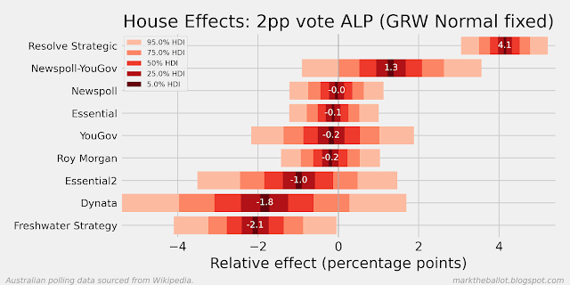
There are two main reasons I have been using Bayesian methods for polling analysis. First, smoothing, so that I can discern the voting intention signal through the fog of noisy and sometimes contradictory opinion polling. Second, I use these methods to detect “house effects”, the tendency of pollsters to systemically (and I assume unintentionally) to favour one political party or the other.
My primary model was built around the notion of a Gaussian Random Walk. This model imagines a hidden daily walk of population voting intention, which only changes a very small amount from day to day. This voting intention is captured imperfectly by opinion polls from time-to-time. The outputs of this model are familiar. We can see the most likely estimate of the population voting intention, as well as the house effects of each pollster. We can either anchor the model to the actual vote at the last election or assume that pollsters are collectively unbiased (ie. collectively the house effects sum to zero).
A quick aside: You will notice in the above voting-intention charts that I have plotted in the background a random selection of 100 of the 10,000 gaussian random walks I drew on in the Bayesian analysis process.
More recently, I have noticed that a few data scientists are using Gaussian Processes to smooth noisy time series data. So, I thought I would give it a go.
A Gaussian Process approach assumes that the data-points that are taken closer together should be more similar than the data-points that are further apart in time. This is expressed in the model using a function (called a kernel) that quantifies how similar data-points that are closer together should be, and a square covariance matrix that captures the degree of similarity between all the data-points one to another using this function. Rather than model voting intention on every day, this approach only models voting intention on polling days. The kernel function I have used is the Exponentiated Quadratic kernel. Diagrammatically, the model is as follows.
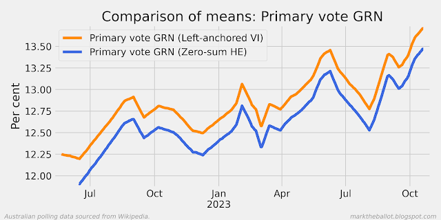
Priors for the model affect how much smoothing will be applied. With a length_scale around 20, the model produces output that is quite like the Gaussian Random Walk above.
I am a little intrigued by the small differences between these last two charts and the first two charts above. Because these are still under development, it is entirely possible that I have made an error somewhere. Nonetheless, a possible explanation for some of the small differences might be the tendency for the GP with certain kernels to revert to the mean. This might explain the slightly higher overall level, and the up-tick at the right end of the series. The GRW does not have a mean-reversion bias.
For the moment, I will prefer the results of the GRW over the new GP approach. However, I will continue to test, develop, and explore the GP model.
The primary vote charts follow for completeness.
For those who are particularly interested, the core code for the model follows. For the complete code, you can check out my GitHub site.
def house_effects_model(inputs: dict[str, Any], model: pm.Model) -> pt.TensorVariable:
    """The house effects model."""

    with model:
        house_effect_sigma = 5.0
        house_effects = pm.ZeroSumNormal(
            "house_effects", sigma=house_effect_sigma, shape=inputs["n_firms"]
        )
    return house_effects


def gp_prior(
    inputs: dict[str, Any],
    model: pm.Model,
    length_scale: Optional[float] = None,
    eta: Optional[float] = None,
) -> pt.TensorVariable:
    """Construct the Gaussian Process (GP) latent variable model prior.
    The prior reflects voting intention on specific polling days.

    Note: Reasonably smooth looking plots only emerge with a lenjth_scale
    greater than (say) 15. Divergences occur when eta resolves as being
    close to zero, (which is obvious when you think about it, but also
    harder to avoid with series that are fairly flat). To address
    these sampling issues, we give the gamma distribution a higher alpha,
    as the mean of the gamma distribution is a/b. And we truncate eta to
    well avoid zero (noting eta is squared before being multiplied by the
    covariance matrix).

    Also note: for quick test runs, length_scale and eta can be fixed
    to (say) 20 and 1 respectively. With both specified, the model runs
    in around 1.4 seconds. With one or both unspecified, it takes about
    7 minutes per run."""

    with model:
        if length_scale is None:
            gamma_hint = {"alpha": 20, "beta": 1}  # ideally a=20, b=1
            length_scale = pm.Gamma("length_scale", **gamma_hint)
        if eta is None:
            eta = pm.TruncatedNormal("eta", mu=1, sigma=5, lower=0.5, upper=20)
        cov = eta**2 * pm.gp.cov.ExpQuad(1, length_scale)
        gp = pm.gp.Latent(cov_func=cov)
        gauss_prior = gp.prior("gauss_prior", X=inputs["poll_day_c_"])
    return gauss_prior


def gp_likelihood(
    inputs: dict[str, Any],
    model: pm.Model,
    gauss_prior: pt.TensorVariable,
    house_effects: pt.TensorVariable,
) -> None:
    """Observational model (likelihood) - Gaussian Process model."""

    with model:
        # Normal observational model
        pm.Normal(
            "observed_polls",
            mu=gauss_prior + house_effects[inputs["poll_firm"]],
            sigma=inputs["measurement_error_sd"],
            observed=inputs["zero_centered_y"],
        )


def gp_model(inputs: dict[str, Any], **kwargs) -> pm.Model:
    """PyMC model for pooling/aggregating voter opinion polls,
    using a Gaussian Process (GP). Note: kwargs allows one to pass
    length_scale and eta to gp_prior()."""

    model = pm.Model()
    gauss_prior = gp_prior(inputs, model, **kwargs)
    house_effects = house_effects_model(inputs, model)
    gp_likelihood(inputs, model, gauss_prior, house_effects)
    return model
Further reading: