Lessons on pooling polls from the 2010 federal election

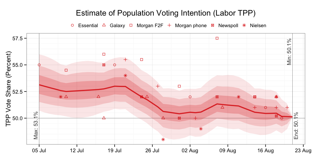
With thanks to the reader who sent me the Galaxy data in the lead-up to the 2010 election, I have re-run the earlier analysis of house effects and the likely pathway for population voting intention.

That final Galaxy poll (52-48 for Labor) is illustrative of the challenge when analysing individual polling statistics immediately prior to an election. The most likely population voting intention pathway (the red line in the above chart) is within the margin of error of (+/-) 3 per cent for the final Galaxy poll. The Galaxy poll was statistically accurate. You cannot ask for more from an individual poll.

However, as we know, the final outcome of 50.12 to 49.88 per cent in Labor's favour produced a hung parliament. If the outcome had been at the centre of the distribution implied in final Galaxy poll, it would have produced a sizable Labor win. The irony is that Galaxy's house effect over the period was slightly pro-Coalition.

If we re-run the above analysis (1) without anchoring the end-point to the election result and (2) if we introduce the constraint that the house effects will sum to zero we get the following plots.

These plots remind us that pooling the polls does not automatically result in an unbiased estimate of the population voting intention. There is no guarantee that house effects will cancel each other out. In this case, the pooled polls were out by 1 percentage point. In 2010 it turned out to be the difference between a hung parliament and a comfortable win for Labor.

How I convert national TPP estimates into likely election outcomes

This is a short methodology discussion on how I generate a possible House of Representatives outcome from a national two-party preferred (TPP) poll estimate. This is not the most sophisticated approach possible (and it will not be the ultimate way I generate these predictions as I refine my models). But, it is what I do at the moment.

The first thing I did was to secure an estimate of the TPP vote for each seat in the 2010 federal election adjusted for boundary changes and redistributions since the 2010 election. I have shamelessly used Antony Green's pendulum for this purpose.

Secondly, building on some of the assumptions Antony made, I thought about how I should handle the treatment of independents (which sit a little outside of the mechanics of a TPP estimate). My current approach is based on the following assumptions (which are not dissimilar to Poliquant's approach):

1. Bob Katter will win Kennedy
2. Andrew Wilkie will win Denison (Labor polling in the Oz 26/06/12, ReachTEL 29/6/12)
3. Adam Bandt will lose Melbourne. [Note: this assumption is a little speculative. It rests on the Liberals changing their preference strategy from their 2010 approach (which they have said they will do). This would  see Liberal preferences flow to Labor:Greens at 67:33 in 2013 rather than the 20:80 flow in  2010. At the 2010 election Labor won 38.1 and the Greens 36.2 per cent of the primary vote. I am not aware of any subsequent polling in the Federal seat of Melbourne; but the Greens lost the 2012 by-election in the related State seat of Melbourne (where Liberals preferenced Labor ahead of Greens)].
4. Rob Oakshott will lose Lyne (Newspoll 24/10/11; ReachTEL 25/8/2011, 20/6/2012)
5. Tony Windsor will lose New England (Newspoll 24/10/11; ReachTEL 19/6/2012) 
6. Peter Slipper's seat of Fisher will be a normal Coalition/Labor contest next election 
7. Craig Thomson's seat of Dobell will be a normal Coalition/Labor contest next election
8. Tony Crook will re-contest O'Connor for the Coalition in a normal Coalition/Labor contest 

I made some tweak's to the pendulum to give effect to these assumptions.

Next I made a quick estimate of the number of seats by calculating the swing from the previous election and summing the probabilities of a win for each of the 150 seats if that swing was applied. The R-code for this function follows. As you can see, it is a short piece of code. The heavy lifting is done by the sum(pnorm(...)) functions in the middle of this code.

seatCountFromTPPbyProbabilitySum <- function(pendulumFile='./files/AntonyGreenTPP.csv', 
    pendulum, LaborTPP) {

    ALP.Outcome.2010 <- 50.12
    swing <- LaborTPP - ALP.Outcome.2010

    if(missing(pendulum)) {
        pendulum <- read.csv(pendulumFile, stringsAsFactors=FALSE)
        pendulum$ALP_TPP <- as.numeric(pendulum$ALP_TPP)
    }
    
    # Note: sd in next line comes from analysis of federal elections since 1996 ...
    ALP = round( sum( pnorm(pendulum$ALP_TPP + swing, mean=50, sd=3.27459) ) )
    
    pc <- pendulum[pendulum$OTHER == 'OTHER', ]
    OTHER = round( sum( pnorm(100 - pc$ALP_TPP - swing, mean=50, sd=3.27459) ) )

    COALITION = 150 - ALP - OTHER # Just to ensure it all adds to 150.

    # return a data frame - makes it easier to ggplot later
    results <-                data.frame(Party='Other',         Seats=OTHER)
    results <- rbind(results, data.frame(Party='Coalition',     Seats=COALITION))
    results <- rbind(results, data.frame(Party=factor('Labor'), Seats=ALP))
    
    return(results)
}

Update: I have updated the model to better manage how I treat Denison.

seatCountFromTPPbyProbabilitySum <- function(pendulumFile='./files/AntonyGreenTPP.csv', 
    pendulum, LaborTPP) {

    ALP.Outcome.2010 <- 50.12
    swing <- LaborTPP - ALP.Outcome.2010

    if(missing(pendulum)) {
        pendulum <- read.csv(pendulumFile, stringsAsFactors=FALSE)
        pendulum$ALP_TPP <- as.numeric(pendulum$ALP_TPP)
    }
    
    # Note: sd in next few lines comes from analysis of federal elections since 1996 ...
    pc <- pendulum[pendulum$OTHER == 'OTHER', ]
    other.raw <- sum( pnorm(100 - pc$ALP_TPP - swing, mean=50, sd=3.27459) )
    OTHER <- round( other.raw )
    carry <- other.raw - OTHER

    # this approach typically favours Labor (probably the right way to go)
    ALP <- round( carry + sum( pnorm(pendulum$ALP_TPP + swing, mean=50, sd=3.27459) ) )
    
    COALITION <- 150 - ALP - OTHER # Just to ensure it all adds to 150.

    # return a data frame - makes it easier to ggplot later
    results <-                data.frame(Party='Other',         Seats=OTHER)
    results <- rbind(results, data.frame(Party='Coalition',     Seats=COALITION))
    results <- rbind(results, data.frame(Party=factor('Labor'), Seats=ALP))
    
    return(results)
}

From this function we can plot a likely election outcome for a given a swing.

To get a more nuanced understanding of a potential election outcome, I undertake a simple Monte Carlo simulation (typically with 100,000 iterations). This is not a Bayesian MCMC approach. It's just a plain old fashioned MC simulation. The R-code for this procedure is more substantial.

storeResult <- function(N, pendulum, individualSeats=FALSE) {
    # Use of R's lexical scoping

    # entry sanity checks ...
    stopifnot(is.numeric(N))
    stopifnot(is.data.frame(pendulum))
    stopifnot(N > 0)
    seatCount <- nrow(pendulum)
    stopifnot(seatCount > 0)

    # sanity checking variables
    count <- 0
    finalised <- FALSE

    # where I store the house wins ...
    ALP <- rep(0, length=seatCount)
    COALITION <- rep(0, length=seatCount)
    OTHER <- rep(0, length=seatCount)
    
    CUM_ALP <- rep(0, length=seatCount)
    CUM_COALITION <- rep(0, length=seatCount)
    
    # where I keep the seat-by-seat wins
    seats <- data.frame(seat=pendulum$SEAT, state=pendulum$STATE, Labor=ALP, 
        Coalition=COALITION, Other=OTHER)

    rememberSim <- function(simResult) {

        # - sanity checker
        stopifnot(!finalised)
        stopifnot(count < N)
        count <<- count + 1
        stopifnot(length(simResult) == seatCount)
    
        # - overall result
        a <- table(simResult)
        ALP[ a[names(a)=='ALP'] ] <<- ALP[ a[names(a)=='ALP'] ] + 1
        COALITION[ a[names(a)=='COALITION'] ] <<- 
            COALITION[ a[names(a)=='COALITION'] ] + 1
        OTHER[ a[names(a)=='OTHER'] ] <<- OTHER[ a[names(a)=='OTHER'] ] + 1
        
        # - seat by seat result
        if(individualSeats) {
            seats$Labor <<- ifelse(simResult == 'ALP', seats$Labor + 1,
                seats$Labor)
            seats$Coalition <<- ifelse(simResult == 'COALITION', 
                seats$Coalition + 1, seats$Coalition)
            seats$Other <<- ifelse(simResult == 'OTHER', seats$Other + 1, 
                seats$Other)
        }
    }
    
    finalise <- function() {
        # sanity checker
        stopifnot(!finalised)
        stopifnot(count == N)
        
        ALP <<- ALP / N
        COALITION <<- COALITION / N
        OTHER <<- OTHER / N
        
        if(individualSeats) {
            seats$Labor <<- seats$Labor / N
            seats$Coalition <<- seats$Coalition / N
            seats$Other <<- seats$Other / N
        }
        
        for(i in 1:seatCount) {
            CUM_ALP[i] <<- 1 - sum(ALP[1:i])
            CUM_COALITION[i] <<- 1 - sum(COALITION[1:i])
        }
                
        finalised <<- TRUE
    }        
    
    results <- function() {
        stopifnot(finalised)
        data.frame(seatsWon=1:nrow(pendulum), Labor=ALP, Coalition=COALITION, 
            Other=OTHER)
    }
        
    cumResults <- function() {
        stopifnot(finalised)
        data.frame(seatsWon=1:nrow(pendulum), Labor=CUM_ALP, Coalition=CUM_COALITION)
    }

    winProbabilities <- function() {
        stopifnot(finalised)
        win <- (floor(seatCount/2) + 1):seatCount
        list(Labor = sum(ALP[win]), Coalition = sum(COALITION[win]))
    }

    seatResults <- function() {
        stopifnot(finalised)
        stopifnot(individualSeats)
        seats
    }
    
    list(rememberSim=rememberSim, finalise=finalise, results=results, cumResults=cumResults,
        seatResults=seatResults, winProbabilities=winProbabilities)
}

## -- similate one Federal election
simulateNationaLResult <- function(pendulum, swing) {
    rawPrediction <- pendulum$ALP_TPP + swing
    probabilisticPrediction <- rawPrediction + rnorm(nrow(pendulum), mean=0, sd=3.27459)
    ifelse(probabilisticPrediction >= 50, 'ALP', pendulum$OTHER)
}

## -- run N simulations of one Federal election outcome
simulateOneOutcome <- function(N=100000, pendulumFile='./files/AntonyGreenTPP.csv',
    pendulum, LaborTPP, individualSeats=FALSE) {

    ALP.Outcome.2010 <- 50.12
    swing <- LaborTPP - ALP.Outcome.2010

    if(missing(pendulum)) {
        pendulum <- read.csv(pendulumFile, stringsAsFactors=FALSE)
        pendulum$ALP_TPP <- as.numeric(pendulum$ALP_TPP)
    }
    
    r <- storeResult(N, pendulum, individualSeats)
    for(i in 1:N) r$rememberSim ( simulateNationaLResult(pendulum, swing) )
    r$finalise()

    invisible(r)
}

From this simulation, there are a few plots I can make:

I am currently working on a state-level frame for converting a series of state TPP estimates to a national outcome for the House of Representatives.

Last Newspoll for 2012

Today's Australian has the last Newspoll for 2012.

Updated poll aggregation estimates

Two polls in the last 24 hours: Both Newspoll and Essential have estimated that the two-party preferred (TPP) vote share at 54 to 46 in the Coalition's favour. I have placed these latest data points into my various aggregation models.

Under the LOESS aggregation (with a 180-day localised regression span) - the current estimate of the ALP TPP population voting intention is 47 per cent. The LOESS regression does not make adjustments for polling house effects. Furthermore, the LOESS approach can be overly influenced by end-points in the data-stream.

Using a Bayesian fixed house-effects model, over a six month span in recognition that house effects can move around over the medium term, the ALP TPP population voting intention is 47.1 per cent. While this model includes a house effect, that effect is distributed around a constant over the period. Furthermore, the model only applies a relative effect with the constraint that the total effect for all of the polling houses sums to zero. At past elections, this has not been the case.

In applying the time-varying house effects model, I use the part of the model that eliminates noise (but hopefully retains signal). This model placed the Labor TPP at 47.4 per cent. Like the previous model, it also assumes that house effects sum to zero (but over six months on average).

Note, the house effects in the next chart are measured in relative terms to the other polling houses over six months.

I translate the current state of the polls to the Coalition winning around 85 or 86 seats.

More on house effects over time

Early last decade, Simon Jackman published his Bayesian approach to poll aggregation. It allowed the house effects (systemic biases) of a polling house to be calibrated (either absolutely in terms of a known election outcome, or relatively against the average of all the other polling houses).

Jackman's approach was two-fold. He theorised that voting intention typically did not change much day-to-day (although his model allows for occasional larger movement in public opinion). On most days, the voting intention of the public is much the same as it was on the previous day. In his model, he identified the most likely path that voting intention took each and every day through the period under analysis. This day-to-day track of likely voting intention then must line up (as best it can) with the published polls as they occurred during this period. To help the modeled day-to-day walk of public opinion line up with the published polls, Jackman's approach assumed that each polling house had a  systemic bias which is normally distributed around a constant number of percentage points above or below the actual population's voting intention.

Jackman's approach works brilliantly over the short run. In the next chart, which is based on a 100,000 simulation of possible walks that satisfies the constraints in the model, we pick out the median pathway for each day over the last six months. The result is a reasonably smooth curve. While I have not labeled the end point in the median series, it was 47.8 per cent.

However, over longer periods, Jackman's model is less effective. The problem is the assumption that the distribution of house effects remains constant over time. This is not the case. In the next chart, we apply the same 100,000 simulation approach as above, but to the data since the last election. The end point for this chart is 47.7 per cent.

It looks like the estimated population voting intention line is more choppy (because the constantly distributed house effects element of the model is contributing less to the analysis over the longer run). Previously I noted that over the last three years, Essential's house effect has moved around somewhat in comparison to the other polling houses.

All of this got me wondering whether it was possible to design a model that identified this movement in house effects over time - on (say) a six month rolling average basis. My idea was to take the median line from Jackman's model and use it to benchmark the polling houses.  I also wondered whether I could then use the newly identified time-varying house-effect to better identify the underlying population voting intention.

The first step of taking a six month rolling average against the original Jackman line was simple as can be seen in the next chart (noting this is a 10,000 run simulation).

However, designing a model where the fixed and variable sides of the model informed each other proved more challenging than I had anticipated (in part because the JAGS program requires the specification of a directed acyclic graph). At first, I could not find an easy way for the fixed effect side of the model to inform variable effects side of the model and for the variable effects side to inform the fixed effects side, without the whole model becoming a cyclical graph.

When I finally solved the problem, a really nice chart for population voting intention popped out the other end (after 2.5 hours of computer time for the 100,000 run simulation).

Also, the six-monthly moving average for the house effects (which is measured against the line) looked a touch smoother (but this may be the result of a 100,000 run versus a 10,000 run for the earlier chart).

This leads me to another observation. A number of other blogs interested in poll aggregation ignore or down-weight the Morgan face-to-face poll series. I have been asked why I use it.

I use the Morgan face to face series because it is fairly consistent in respect of the other polls. It is a bit like comparing a watch that is consistently five minutes slow with a watch that is sometimes a minute or two fast and at other times a minute or two slow, but which moves randomly between theses two states. A watch that is consistently slow is more informative once it has been benchmarked than a watch that might be closer to the actual time, but whose behaviour around the actual time is random. In short, I think the people who ignore or down-play this Morgan series are not taking advantage of really useful information.

Back to the model: All of the volatility ended up in the variable effects daily walk, which is substantially influenced by the outliers.

For the nerds: My JAGS code for this is a bit more complicated than for earlier models. The variables y and y2 are the polling observations over the period (the series are identical - this is how I ensured the graph was acyclical). The observations are ordered in date order. The lower and upper variables map the range of the six-month centred window for estimating the variable effects against the fixed effects (this is calculated in R before handing to JAGS for the MCMC simulation). The lines marked with a triple $ sign are the lines that allow the fixed and variable elements of the model to inform each other.

    model {
        ## -- temporal model for voting intention (VI)
        for(i in 2:PERIOD) { # for each day under analysis ...
            VI[i] ~ dnorm(VI[i-1], walkVIPrecision)     # fixed effects walk
            VI2[i] ~ dnorm(VI2[i-1], walkVIPrecision2)  # $$$
        }
        
        ## -- initial fixed house-effects observational model
        for(i in 1:NUMPOLLS) { # for each poll result ...
            roundingEffect[i] ~ dunif(-houseRounding[i], houseRounding[i])
            yhat[i] <- houseEffects[ house[i] ] + VI[ day[i] ] + roundingEffect[i]  ## system
            y[i] ~ dnorm(yhat[i], samplePrecision[i])                               ## distribution
        }
        
        ## -- variable effects 6-month window adjusted observational model
        for(i in 1:NUMPOLLS) { # for each poll result ...
            count[i] <- sum(house[ lower[i]:upper[i] ] == house[i])
            adjHouseEffects[i] <- sum( (y[ lower[i]:upper[i] ] - VI[ day[i] ]) *
                (house[ lower[i]:upper[i] ] == house[i]) ) / count[i]
            roundingEffect2[i] ~ dunif(-houseRounding[i], houseRounding[i])     # $$$
            yhat2[i] <- adjHouseEffects[i] + VI2[ day[i] ] + roundingEffect2[i] # $$$
            y2[i] ~ dnorm(yhat2[i], samplePrecision[i])                         # $$$
        }
        
        ## -- point-in-time sum-to-zero constraint on constant house effects
        houseEffects[1] <- -sum( houseEffects[2:HOUSECOUNT] )

        ## -- priors
        for(i in 2:HOUSECOUNT) { ## vague normal priors for house effects
            houseEffects[i] ~ dnorm(0, pow(0.1, -2))
        }

        sigmaWalkVI ~ dunif(0, 0.01)            ## uniform prior on std. dev.  
        walkVIPrecision <- pow(sigmaWalkVI, -2) ##   for the day-to-day random walk
        VI[1] ~ dunif(0.4, 0.6)                 ## initialisation of the voting intention daily walk

        sigmaWalkVI2 ~ dunif(0, 0.01)             ## $$$  
        walkVIPrecision2 <- pow(sigmaWalkVI2, -2) ## $$$
        VI2[1] ~ dunif(0.4, 0.6)                  ## $$$
    }

I suspect this is more complicated than it needs to be; any help in simplifying the approach would be appreciated.

LOESS and Bayes: end-points currently in agreement

A 180 day localised regression (LOESS) of the same polling data as feed to my Bayesian aggregator has the same end-point (even if the journey to that point is not quite the same).

New blog and an updated poll aggregation

Welcome to my new blog. It is the child of Mark the Graph, where I have been exploring statistics and the economy.  The focus for this new blog is on rigorous, impartial analyses of election polling data. I am particularly interested in the application of Bayesian techniques to polling data.

We begin with the Bayesian aggregation of polling data (now including Galaxy). This latest aggregation is suggesting a slight move away from the government in recent weeks.

The weekly Bayesian poll aggregation: 48-52

I am now in a position to publish a weekly aggregation of the national opinion polls on voting intention. The headline message from the first aggregation: following an improvement in Labor's fortunes between July and mid October, national two-party preferred (TPP) voting intention has flat-lined since mid-October. If we assume that all of the house effects sum to zero over time, then the current outcome is 48.2 to 51.8 in the Coalition's favour.

At the moment, I am aggregating five separate polls: Essential, Morgan (treating the face-to-face and phone polls separately), Newspoll and Nielsen. The polls appear in the aggregation on the mid-point date of the polling period. Because Essential's weekly polls appear twice in their weekly report (as a fortnightly aggregation), I only use every second Essential report (beginning with the most recent).

This aggregation assumes that the systemic biases across the five polling streams sum to zero. Because this is an unrealistic assumption, I also produce a chart on the relative house effects of the polling houses for the period under analysis. The distance from the house median and the zero line indicates the biases applied to or subtracted from polling houses in the above chart. (Note: These will move around over time.) You can then decide whether the estimate of the national population voting intention in the first chart needs to be adjusted up or down a touch.

As a rough indication, this outcome would see the following probabilities for the minimum number of seats won.

This is not the end point in my opinion poll analytical efforts. I have started work on a Bayesian state-space model for Australia's five most populous states. This should allow for a more accurate outcome prediction on a state-by-state basis.

House effects over time

Yesterday, I looked at the house effects in the opinion polls following the elevation of Julia Gillard up until the 2010 Federal Election (actually a slightly narrower period: from 5 July to 21 August 2010). The key charts were as follows.

The house effect difference between the polling houses can be summarised in terms of relative percentage point differences as follows:

• Between Morgan face-to-face and Essential: 1.83 percentage points 
• Between Essential and Morgan phone: 0.17 percentage points 
• Between Morgan phone and Newspoll: 0.43 percentage points 
• Between Newspoll and Nielsen: 0.78 percentage points 

Unfortunately, apart from elections we cannot  benchmark the opinion polls to the actual population wide voting intention. We can, however, benchmark the polls against each other. I have adjusted my JAGS code so that the house affects must sum to zero over the period under analysis. This yields the next two charts covering the same period as the previous charts.

While this sum-to-zero constraint results in a biased estimate of population voting intentions (it's around 1 per cent pro-Labor compared with the initial election-outcome anchored analysis), the relative house effects remain largely unchanged in the analysis for the period:

• Between Morgan face-to-face and Essential: 1.83 percentage points
• Between Essential and Morgan phone: 0.16 percentage points
• Between Morgan phone and Newspoll: 0.44 percentage points
• Between Newspoll and Nielsen: 0.77 percentage points

In plain-English - the shape of the population voting curve is much the same between the two-approaches; what has changed is the vertical position of that curve.

If house effects were constant over time, it would be easy to apply this bench-marked effect to future polls. Unfortunately house effects are not constant over time. In the next three sets of charts we can see that the relativities move around - some quite markedly. The charts span three roughly one-year periods: Kevin Rudd's last 12 months as leader; calendar year 2011; and calendar year 2012.

The intriguing question I am left pondering is whether Essential has made changes to its in-house operations that have affected its relative house effects position. It also has me wondering how much I should adjust (move up or move down) the unadjusted estimate of population voting intention to get a more accurate read on the mood of the nation.

And the most recent three months ... which might just be a pretty good proxy for how the population voting trend is tracking at the moment.

Caveat: this analysis is a touch speculative.  If you see errors in my data or analytical approach, or have additional data you can give me, please drop me a line and I will re-run the analysis.

JAGS code:

    model {
        ## -- observational model
        for(i in 1:NUMPOLLS) { # for each poll result ...
            roundingEffect[i] ~ dunif(-houseRounding[i], houseRounding[i])
            yhat[i] <- houseEffect[house[i]] + walk[day[i]] + roundingEffect[i] # system
            y[i] ~ dnorm(yhat[i], samplePrecision[i]) # distribution
        }
            
        ## -- temporal model
        for(i in 2:PERIOD) { # for each day under analysis ...
            walk[i] ~ dnorm(walk[i-1], walkPrecision) # AR(1)
        }

        ## -- sum-to-zero constraint on house effects
        houseEffect[1] <- -sum( houseEffect[2:HOUSECOUNT] )
        zeroSum <- sum( houseEffect[1:HOUSECOUNT] ) # monitor

        ## -- priors
        sigmaWalk ~ dunif(0, 0.01)          ## uniform prior on std. dev.  
        walkPrecision <- pow(sigmaWalk, -2) ##   for the day-to-day random walk
        walk[1] ~ dunif(0.4, 0.6)           ## initialisation of the daily walk

        for(i in 2:HOUSECOUNT) { ## vague normal priors for house effects
            houseEffect[i] ~ dnorm(0, pow(0.1, -2))
        }
    }

House effects: a first look at the 2010 election

Following the 2004 and 2007 Federal Elections, Professor Simon Jackman published on the "house effects" of Australia's polling houses. Unfortunately, I could not find a similar analysis for the 2010 election, so for this blog I have developed a preliminary exploration of the issue.

For Jackman, house effects are the systemic biases that affect each pollster's published estimate of the population voting intention. He assumed that each published estimate from a polling house typically diverged from the from real population voting intention by a constant number of percentage points (on average and over time).

To estimate these house effects, Jackman developed a two-part model where each part of the model informed the other. Rather than outline a formal Bayesian description for Jackman's approach (with a pile of Greek letters and twiddles), I will talk through the approach.

The first part of Jackman's approach was a temporal model. It assumed that on any particular day the real population voting intention was much the same as it was on the previous day. To enable the individual house effects to be revealed, the model is anchored to the actual outcome on the election day (for the 2010 Election, the anchor would be 50.12 per cent in Labor's favour).

In the second part - the observational model - the voting intention published by a polling house for a particular date is assumed to encompass the actual population voting intention, a house effect and the margin of error for the poll.

Using a Markov chain Monte Carlo technique, Jackman identified the most likely day-to-day pathway for the temporal model for each day under analysis and the most likely house effects given the data from the observational model.

I have replicated Professor Jackman's approach in respect of the 2010 election, with a small modification to account for the different approaches to rounding taken by each polling house. I have used the TPP estimates published by the houses. Like Jackman, I used the down-rounded, mid-point date for those polls that spanned a period. As the weekly Essential reports typically aggregate two polls over a fortnight (resulting in individual weekly polls appearing twice in the Essential report data stream), I ensured that the weekly polls only appeared once in the input data to the model. Typically, this meant excluding every second Essential report.

Unfortunately, I do not have polling data for Galaxy in the lead up to the 2010 Election (if someone wants to send it to me I would be greatly appreciative). Also, I don't have the sample sizes for for all of the polls, and I have used estimates based on reasonable guesses. Consequently, this analysis must be considered incomplete. Nonetheless, my initial results follow.

In this first chart, we have the hidden temporal model estimate for each day between 5 July 2010, and the election on 21 August 2010. The red line is the median estimate from a 100,000 simulation run. The darkest zone represents the 50% credibility zone. The outer edges of the second darkest zone expands on the 50% zone to highlight the 80% credibility zone. The outer edges of the lightest zone similarly shows the 95% credibility zone.

The second chart is the estimated house effects for five of Australia's polling houses going into the 2010 Federal election. The shading in this chart has the same meaning as the previous chart. A negative value indicates that the house effect favours the Coalition. A positive value favours Labor.

The JAGS code for this analysis follows.

    model {
        ## -- observational model
        for(i in 1:length(y)) { # for each poll result ...
            roundingEffect[i] ~ dunif(-houseRounding[i], houseRounding[i])
            mu[i] <- houseEffect[house[i]] + walk[day[i]] + roundingEffect[i] # system
            y[i] ~ dnorm(mu[i], samplePrecision[i]) # distribution
        }
        
        ## -- temporal model
        for(i in 2:period) { # for each day under analysis ...
            walk[i] ~ dnorm(walk[i-1], walkPrecision) # AR(1)
        }

        ## -- priors
        sigmaWalk ~ dunif(0, 0.01)          ## uniform prior on std. dev.  
        walkPrecision <- pow(sigmaWalk, -2) ##   for the day-to-day random walk
        walk[1] ~ dunif(0.4, 0.6)           ## initialisation of the daily walk

        for(i in 1:5) {                     ## vague normal priors for house effects
            houseEffect[i] ~ dnorm(0, pow(0.1, -2))
        }
    }