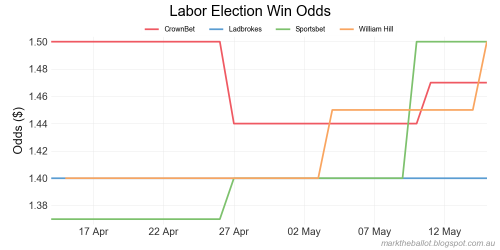
Last Saturday's by-election results have not really shifted punter sentiments. The punters think Shorten and Labor more likely to win the next Federal election, but it is actually a reasonably close race. This has not changed hugely since mid April 2018.
When I look at betting markets, I tend to treat any movement of less than five percentage points as not significant. The bookmaker's over-round and the reality that these are thin markets means that small movements of one or two percentage points are more likely to be noise rather than signal.
If we average the house results for a clearer picture, we can see that the mean win probability for the Coalition since I have been following this matter has largely been between 35 and 40 per cent. (ignoring the fact that I did not collect odds in the first two weeks of July while I was taking a holiday).
The raw charts follow.
Wednesday, August 1, 2018
Saturday, June 30, 2018
Betting Market Update
This morning's quick look at betting markets sees some movement at Sportsbet.
| House | Coalition Odds ($) | Labor Odds ($) | Coalition Win Probability (%) | |
|---|---|---|---|---|
| 2018-06-30 | CrownBet | 2.25 | 1.47 | 39.52 |
| 2018-06-30 | Ladbrokes | 2.50 | 1.40 | 35.90 |
| 2018-06-30 | Sportsbet | 2.10 | 1.45 | 40.85 |
| 2018-06-30 | William Hill | 2.55 | 1.50 | 37.04 |
Sunday, June 24, 2018
Poll aggregation update
There were two new polls published last week, from Newspoll and Essential, both of which estimated the Coalition has 48 and Labor has 52 per cent of the two-party preferred (TPP) vote share. The aggregation of all polls has the Coalition on 47.9 and Labor on 52.1.
Cross checking this result against some simple moving averages, constrained such that house effects sum to zero, yields the following. Most of these moving averages are still factoring in the up-swing since November last year. I have mentioned before that these moving averages are less reliable around the endpoints than the Bayesian model.
My suspicion is that the Coalition's up-swing since late last year has run its course and we have seen fairly stable numbers for a month and a half or so now at around 48 per cent TPP for the Coalition.
Turning to the primary vote estimates we have ...
In separate analysis, we can look at the Pauline Hanson One Nation Party results, which are included in the Other Parties primary vote chart immediately above ...
The TPP estimate from the logit primary vote model is less favourable to the Coalition than the published polls, using the preference flows from the most recent elections.
Cross checking this result against some simple moving averages, constrained such that house effects sum to zero, yields the following. Most of these moving averages are still factoring in the up-swing since November last year. I have mentioned before that these moving averages are less reliable around the endpoints than the Bayesian model.
My suspicion is that the Coalition's up-swing since late last year has run its course and we have seen fairly stable numbers for a month and a half or so now at around 48 per cent TPP for the Coalition.
Turning to the primary vote estimates we have ...
In separate analysis, we can look at the Pauline Hanson One Nation Party results, which are included in the Other Parties primary vote chart immediately above ...
The TPP estimate from the logit primary vote model is less favourable to the Coalition than the published polls, using the preference flows from the most recent elections.
Saturday, June 23, 2018
The dramas of a daily web scraper
I have a set of web scraping programs I run every day to update the data for my election betting market series.
These programs are very short, typically 20 to 30 lines of Python code. But they are highly idiosyncratic. They break when a bookmaker updates the way in which it serves up web pages. My usual approach when this happens is to do a quick fix as soon as I see one of my scrapers has failed.
Sometime between Tuesday morning and Wednesday morning this week, Sportsbet updated the way in which it serves up web pages. It was a dramatic change. Sportsbet want from using bog standard HTML to a JavaScript page that dynamically creates the HTML on the fly.
This necessitated a different approach to web scraping. And I only found the time today (Saturday afternoon) to update the Sportsbet web scraper.
In the mean time, it looks like the odds have moved at Sportsbet.
Sportsbet now has the Coalition in the best position it has been in since I started my daily monitoring of odds for the winner of the next Australian federal election. In case you are wondering, the next federal election is most likely to be held in the first half of 2019, but it could happen earlier.
These programs are very short, typically 20 to 30 lines of Python code. But they are highly idiosyncratic. They break when a bookmaker updates the way in which it serves up web pages. My usual approach when this happens is to do a quick fix as soon as I see one of my scrapers has failed.
Sometime between Tuesday morning and Wednesday morning this week, Sportsbet updated the way in which it serves up web pages. It was a dramatic change. Sportsbet want from using bog standard HTML to a JavaScript page that dynamically creates the HTML on the fly.
This necessitated a different approach to web scraping. And I only found the time today (Saturday afternoon) to update the Sportsbet web scraper.
In the mean time, it looks like the odds have moved at Sportsbet.
Sportsbet now has the Coalition in the best position it has been in since I started my daily monitoring of odds for the winner of the next Australian federal election. In case you are wondering, the next federal election is most likely to be held in the first half of 2019, but it could happen earlier.
Sunday, June 10, 2018
Poll update
The latest aggregation follows. It treats the Newspolls since December 2017 as a different series to the earlier Newspolls. I have split Newspoll into two series on the basis of its treatment of One Nation preferences. The current two-party preferred (TPP) estimate, based on the assumption that house effects balance out on average, sees the Coalition on 47.8 per cent to Labor's election winning position of 52.2 per cent.
As a cross check, let's look at how this compares with a number of moving averages, which have been similarly adjusted on the assumption that house effects balance out on average. Both the LOWESS-91 and and Bayesian hierarchical model (above) suggest that the Coalition's poll position may have peaked and is now trending down.The moving averages are slower than the Bayesian to respond to changes in public opinion. They can also exaggerate the end point position.
We can also compare the estimated house biases from the various moving averages compared with the Bayesian model above.
Let's move to the TPP analysis based on primary votes and preference flows at the last Federal election. This use of preference flows is less favourable to the Coalition than the latest flows at Newspoll. We are not seeing a downturn in any of these series. This might be the additional constraints in the primary vote model makes it less responsive to chnages in public sentiment. But this might be because the model does not take account of One Nation preference flows separately from other parties in the others category.
The primary vote share estimates follow.
Separating One Nation from Other above ... we can see a party that appears to be in decline, and well down on its peak in early 2017.
As a cross check, let's look at how this compares with a number of moving averages, which have been similarly adjusted on the assumption that house effects balance out on average. Both the LOWESS-91 and and Bayesian hierarchical model (above) suggest that the Coalition's poll position may have peaked and is now trending down.The moving averages are slower than the Bayesian to respond to changes in public opinion. They can also exaggerate the end point position.
We can also compare the estimated house biases from the various moving averages compared with the Bayesian model above.
| Essential | Ipsos | Newspoll | Newspoll2 | ReachTEL | Roy Morgan | YouGov | Iter | Sum Errors Squared | |
|---|---|---|---|---|---|---|---|---|---|
| Model | |||||||||
| HMA-181 | -0.805492 | -0.864758 | -0.792727 | 0.073339 | -0.324017 | 0.511941 | 2.201714 | 22 | 0.008374 |
| HMA-365 | -0.781727 | -0.742800 | -0.723322 | 0.054020 | -0.300477 | 0.293336 | 2.200970 | 20 | 0.009416 |
| LOWESS-91 | -0.801099 | -0.883610 | -0.807314 | 0.132668 | -0.290249 | 0.443300 | 2.206304 | 19 | 0.008246 |
| LOWESS-181 | -0.803521 | -0.804463 | -0.770847 | 0.111452 | -0.311898 | 0.369247 | 2.210029 | 16 | 0.009263 |
Let's move to the TPP analysis based on primary votes and preference flows at the last Federal election. This use of preference flows is less favourable to the Coalition than the latest flows at Newspoll. We are not seeing a downturn in any of these series. This might be the additional constraints in the primary vote model makes it less responsive to chnages in public sentiment. But this might be because the model does not take account of One Nation preference flows separately from other parties in the others category.
The primary vote share estimates follow.
Separating One Nation from Other above ... we can see a party that appears to be in decline, and well down on its peak in early 2017.
Monday, May 28, 2018
Newspoll adjustment
The latest Newspoll estimated the Coalition would win 48 per cent, and Labor 52 per cent of the two-party preferred (TPP) vote share if an election was held now. Not a surprising result, and consistent with many other polls over recent months.
However it prompted me to do something about my Bayesian Hidden Markov Model. As many of you would know: in December 2017, Newspoll changed the way it allocates preferences in respect of the One Nation Party (see Poll Buldger, and Kevin Bonham). My Bayesian model assumes each polling house has an unchanging methodology. Clearly, we now know this is not the case. Newspoll has increased its preference flow from One Nation primary votes to the Coalition TPP vote share by an undisclosed amount. As a result, the Coalition TPP has improved by around one percentage point on average in the Newspoll series since December 2017. The easy model fix is to treat these later Newspoll results as a separate series.
Let's start today's TPP charts with what they would have been had I not changed the treatment of Newspoll within the model. The thing to note here is that the overall increase from low-point to now is 0.9 percentage points.
Now, let's look at the results when we treat the post 1 December 2017 Newspolls as being a different series. The increase from the low-point to now is little changed in the model. Treating Newspoll as a single series (with the same data) the increase from the low-point was 0.9 percentage points, and treating Newspoll as two series, this increase is 0.8 percentage points.
The new treatment also changes the vertical positioning of the lines, but this is largely an artifact of the sum to zero constraint on house effects across the houses.
More interestingly, the new treatment reveals a change in the estimated pro-Coalition bias for Newspoll of (almost exactly) one percentage point (being the difference between -0.8295 and +0.1712).
What this suggests is that today's result might have been closer to 47 to 53, Coalition to Labor, if Newspoll had not changed its preference flow methodology. I happen to think on balance that Newspoll's newer methodology is the more accurate. It certainly reflects recent state government election preference flows. But given One Nation's history I have one (huge) caveat. If, come the election, One Nation decides to preference against the Coalition on its how to vote cards, then I suspect the recent state elections will not mean a thing.
Usual acknowledgement: the data for this analysis comes from Wikipedia.
However it prompted me to do something about my Bayesian Hidden Markov Model. As many of you would know: in December 2017, Newspoll changed the way it allocates preferences in respect of the One Nation Party (see Poll Buldger, and Kevin Bonham). My Bayesian model assumes each polling house has an unchanging methodology. Clearly, we now know this is not the case. Newspoll has increased its preference flow from One Nation primary votes to the Coalition TPP vote share by an undisclosed amount. As a result, the Coalition TPP has improved by around one percentage point on average in the Newspoll series since December 2017. The easy model fix is to treat these later Newspoll results as a separate series.
Let's start today's TPP charts with what they would have been had I not changed the treatment of Newspoll within the model. The thing to note here is that the overall increase from low-point to now is 0.9 percentage points.
Now, let's look at the results when we treat the post 1 December 2017 Newspolls as being a different series. The increase from the low-point to now is little changed in the model. Treating Newspoll as a single series (with the same data) the increase from the low-point was 0.9 percentage points, and treating Newspoll as two series, this increase is 0.8 percentage points.
The new treatment also changes the vertical positioning of the lines, but this is largely an artifact of the sum to zero constraint on house effects across the houses.
More interestingly, the new treatment reveals a change in the estimated pro-Coalition bias for Newspoll of (almost exactly) one percentage point (being the difference between -0.8295 and +0.1712).
What this suggests is that today's result might have been closer to 47 to 53, Coalition to Labor, if Newspoll had not changed its preference flow methodology. I happen to think on balance that Newspoll's newer methodology is the more accurate. It certainly reflects recent state government election preference flows. But given One Nation's history I have one (huge) caveat. If, come the election, One Nation decides to preference against the Coalition on its how to vote cards, then I suspect the recent state elections will not mean a thing.
Usual acknowledgement: the data for this analysis comes from Wikipedia.
Tuesday, May 15, 2018
A month at the betting market
I have been following the Australian Federal Election betting market for a month now. Not a lot has happened in that month. Across the four houses I regularly sample, punters think that Labor has a 63 per cent chance of winning the next election and the Coalition a 37 per chance. On 15 April, when I started collecting odds from these four houses, it was 65 and 35 per cent.
Friday, May 4, 2018
May poll aggregate update
Another month has passed, so it is time to update the poll aggregate. Let's start with a list of the recent poll results, sourced from the Wikipedia page on the next federal election.
Tossing these results into the two-party preferred aggregation reveals.
This can be compared with my simplified aggregation models using Henderson moving averages (HMA) and Locally Weighted Scatter-plot Smoothing (LOWESS). Both of these models can do strange things at the end points. Given the data, I suspect they are a touch over-enthusiastic for the Coalition come the end of April 2018.
Collectively we can see that the Coalition's fortunes continued their rise through April. Nonetheless, if an election was held now, the most likely outcome would be a sizable Labor victory.
Moving to the primary voting intention results.
Collectively, the implied two-party preferred (TPP) results for the Coalition follow. Unlike the TPP charts above, calculating the TPP results directly from the primary vote sees a stagnating TPP. I suspect the issue here is partly affected by Newspoll's change in methodology for attributing preference flows for One Nation. While I can understand Newspoll's decision to increase the One Nation to Coalition preference flows (based on preference flows at the recent Qld and WA state elections), the changed methodology is inconsistent with my models. I will need to think about this some more.
Speaking of One Nation, there has been a slow decline in its vote share over recent months.
| MidDate | Firm | L/NP | ALP | GRN | ONP | OTH | TPP L/NP | TPP ALP | |
|---|---|---|---|---|---|---|---|---|---|
| 1 | 2018-04-30 | ReachTEL | 36.0 | 35.0 | 11.0 | 6.0 | 12.0 | 48.0 | 52.0 |
| 2 | 2018-04-20 | Essential | 37.0 | 36.0 | 11.0 | 8.0 | 8.0 | 47.0 | 53.0 |
| 3 | 2018-04-22 | Newspoll | 38.0 | 37.0 | 9.0 | 7.0 | 9.0 | 49.0 | 51.0 |
| 4 | 2018-04-06 | Essential | 38.0 | 37.0 | 10.0 | 7.0 | 8.0 | 47.0 | 53.0 |
| 5 | 2018-04-06 | Newspoll | 38.0 | 37.0 | 10.0 | 7.0 | 8.0 | 48.0 | 52.0 |
| 6 | 2018-04-04 | Ipsos | 36.0 | 34.0 | 12.0 | NaN | 18.0 | 48.0 | 52.0 |
Tossing these results into the two-party preferred aggregation reveals.
This can be compared with my simplified aggregation models using Henderson moving averages (HMA) and Locally Weighted Scatter-plot Smoothing (LOWESS). Both of these models can do strange things at the end points. Given the data, I suspect they are a touch over-enthusiastic for the Coalition come the end of April 2018.
Collectively we can see that the Coalition's fortunes continued their rise through April. Nonetheless, if an election was held now, the most likely outcome would be a sizable Labor victory.
Moving to the primary voting intention results.
Collectively, the implied two-party preferred (TPP) results for the Coalition follow. Unlike the TPP charts above, calculating the TPP results directly from the primary vote sees a stagnating TPP. I suspect the issue here is partly affected by Newspoll's change in methodology for attributing preference flows for One Nation. While I can understand Newspoll's decision to increase the One Nation to Coalition preference flows (based on preference flows at the recent Qld and WA state elections), the changed methodology is inconsistent with my models. I will need to think about this some more.
Speaking of One Nation, there has been a slow decline in its vote share over recent months.
Wednesday, April 25, 2018
Simple poll aggregation models
I have played some more with my simplified poll aggregation models using Henderson moving averages (HMA) and Locally Weighted Scatter-plot Smoothing (LOWESS). I fit the smoothed curve taking account of house biases (that is, the systemic tendency for a pollster to favour one house or the other). The models are fit iteratively, with the objective of adjusting the estimated house effects to minimize the sum of the errors squared for the fit. I have also compared these models with the Hierarchical Bayesian model I use.
Cutting to the chase: the plot of the various aggregation models follows. Just under the plot heading you can see the end-point for each of the models (as at 22 April 2018). As usual, the input data for these models comes from the Wikipedia page on the Next Australian Federal Election.
The estimated house biases (the first six columns expressed in pro-Coalition percentage points) for each model (the rows) are in the next table. Note, these are relative house effects as the rows have been constrained to sum to zero. The "Iter" column is the number of iterations taken to produce this estimate. The "Sum Errors Squared" column is the sum of the errors squared, noting that within the model these are calculated from proportions (between 0 and 1) and not percentage points (between 0 and 100).
This compares well with the Hierarchical Bayesian model:
The updated code follows.
Cutting to the chase: the plot of the various aggregation models follows. Just under the plot heading you can see the end-point for each of the models (as at 22 April 2018). As usual, the input data for these models comes from the Wikipedia page on the Next Australian Federal Election.
The estimated house biases (the first six columns expressed in pro-Coalition percentage points) for each model (the rows) are in the next table. Note, these are relative house effects as the rows have been constrained to sum to zero. The "Iter" column is the number of iterations taken to produce this estimate. The "Sum Errors Squared" column is the sum of the errors squared, noting that within the model these are calculated from proportions (between 0 and 1) and not percentage points (between 0 and 100).
| Essential | Ipsos | Newspoll | ReachTEL | Roy Morgan | YouGov | Iter | Sum Errors Squared | |
|---|---|---|---|---|---|---|---|---|
| Model | ||||||||
| HMA-181 | -0.845100 | -0.568599 | -0.615695 | -0.408452 | 0.278507 | 2.159338 | 13 | 0.008061 |
| HMA-365 | -0.832409 | -0.485705 | -0.589923 | -0.401716 | 0.150488 | 2.159266 | 12 | 0.008920 |
| LOWESS-91 | -0.818754 | -0.554349 | -0.604249 | -0.403321 | 0.216127 | 2.164546 | 13 | 0.008110 |
| LOWESS-181 | -0.826693 | -0.475102 | -0.577678 | -0.413161 | 0.169364 | 2.123270 | 12 | 0.009222 |
This compares well with the Hierarchical Bayesian model:
The updated code follows.
# PYHTON: iterative data fusion:
# using Henderson Moving Averages (HMA)
# and Locally Weighted Scatterplot Smoothing (LOWESS)
# with a sum-to-zero adjustment for House biases
import pandas as pd
import numpy as np
from numpy import dot
import matplotlib.pyplot as plt
import matplotlib.dates as mdates
import statsmodels.api as sm
lowess = sm.nonparametric.lowess
import sys
sys.path.append( '../bin' )
from mg_plot import mg_min_max_end
from Henderson import Henderson
plt.style.use('../bin/markgraph.mplstyle')
# --- key constants
HMA_PERIODS = [181, 365] # days
LOWESS_PERIODS = [91, 181] # days
MODALITIES = ['HMA', 'LOWESS']
graph_dir = './Graphs/'
graph_leader = 'FUSION-'
intermediate_data_dir = "./Intermediate/"
# --- Functions
def note_house_effects(effects, Houses, mode, period,
iter_count, current_sum):
''' For each iteration we record the results. This function compiles
the results into a single row DataFrame, which will be appended
to the iteration history DataFrame
effects: is a column vector of house effects that was applied
Houses: is a list of Houses
mode: is a mode in 'HMA' or 'LOWESS'
iter_count: is the iteration count as an integer
current_sum: is the error squared sum as a float
returns: a Pandas DataFrame with one row
'''
house_effects = pd.DataFrame([effects.T[0]],
columns=Houses, index=[iter_count])
house_effects['Iterations'] = iter_count
house_effects['Model'] = '{}-{}'.format(mode, period)
house_effects['Error Sq Sum'] = [current_sum]
house_effects['Effects Sq Sum'] = dot(effects.T, effects)[0]
return house_effects
def interpolate_and_smooth(x):
''' interpolate missing data in a series then apply
a 21-term moving average - with smaller moving averages
at the end of the series.
x: a Pandas Series
returns: a Pandas Series
'''
# set up smoothers - note centre weighting in 7- and 21-term MA
smoother21 = np.array([1,1,2,2,3,3,3,3,3,3,3,3,3,3,3,3,3,2,2,1,1])
smoother21 = smoother21 / np.sum(smoother21)
smoother7 = np.array([1,2,3,3,3,2,1]) # 7-term MA
smoother7 = smoother7 / np.sum(smoother7)
smoother3 = np.array([1,1,1])
smoother3 = smoother3 / np.sum(smoother3)
x = x.interpolate()
# calculate smoothers
s21 = x.rolling(window=len(smoother21), min_periods=len(smoother21),
center=True).apply(func=lambda x: (x * smoother21).sum())
s7 = x.rolling(window=len(smoother7), min_periods=len(smoother7),
center=True).apply(func=lambda x: (x * smoother7).sum())
s3 = x.rolling(window=len(smoother3), min_periods=len(smoother3),
center=True).apply(func=lambda x: (x * smoother3).sum())
# fix the end data from smoothed to less smoothed to unsmoothed
s = s7.where(s21.isnull(), other=s21)
s = s3.where(s.isnull(), other=s)
s = x.where(s.isnull(), other=s)
return(s)
def estimate_hidden_states(ydf, mode, period, n_days):
''' This function takes the house-effect adjusted y values and
estimates a hidden vote share for each day under analysis using
moving averages to give a smooth result.
ydf: is a DataFram of y values,
with cols: Day and adjusted_y
mode: is a MODALITY string - either 'HMA' or 'LOWESS'
period: in days - the span for the moving average
returns: a pandas Series indexed by days
'''
# --- plot known data points and interpolate the in-between days
# where more than one poll on a day, average those polls.
hidden_state = pd.Series(np.array([np.nan] * n_days))
for day in ydf['Day'].unique():
result = ydf[ydf['Day'] == day]
hidden_state[day] = result['adjusted_y'].mean()
# --- apply the HMA or LOWESS smoothing
if mode == 'HMA':
# HMA requires data points for all x values
# therefore we interpolate first
hidden_state = interpolate_and_smooth(hidden_state)
hidden_state = Henderson(hidden_state, period)
elif mode == 'LOWESS':
# LOWESS does not require data points for all x values
hidden_state = pd.Series(
lowess(hidden_state, hidden_state.index, frac=period/n_days,
return_sorted=False))
hidden_state = interpolate_and_smooth(hidden_state)
else:
assert(False)
return hidden_state
def calculate_house_effects(Houses, ydf, hidden_state):
''' For a curve generated by the estimate_hidden_states function,
calculate the zero-sum constrained house effects for each pollster
Houses: is a list of pollsters
ydf: is a pandas DataFrame of y values/attributes,
with columns y, Day and Firm
returns: a column vector of house effects
'''
new_effects = []
for h in Houses:
count = 0
sum = 0
result = ydf[ydf['Firm'] == h]
for index, row in result.iterrows():
sum += hidden_state[row['Day']] - row['y']
count += 1.0
new_effects.append(sum / count)
new_effects = pd.Series(new_effects)
new_effects = new_effects - new_effects.mean() # sum to zero
effects = new_effects.values
effects.shape = len(effects), 1 # it's a column vector
return effects
def sum_error_squared(hidden_state, ydf):
''' For a curve generated by the estimate_hidden_states function,
calculate the sum of the errors-squared for the y observations
hidden_state: a pandas Series indexed by days
ydf: is a pandas DataFrame of y values/attributes,
with columns Day and adjusted_y
returns: a float
'''
dayValue = hidden_state[ydf['Day']]
dayValue.index = ydf.index
e_row = (dayValue - ydf['adjusted_y']).values # row vector
return dot(e_row, e_row.T)
def get_minima(history):
''' Return the minimum sum of errors-squared from the iteration
history DataFrane
history: pandas DataFrame of all iterations to now
returns: minimum value for the sum of errors squared
'''
return history['Error Sq Sum'].min()
def get_details(search, history, Houses):
''' Find the details in the iteration history DataFrame for
a specific search value. The search term is the value of
sum errors squared being sought (typically a minimum)
search: the value of sum errors squared being sought
history: pandas DataFrame of all iterations to now
Houses: is a list of pollsters
returns: (iter_num, effects) - found selected effects in history
'''
effects = history[history['Error Sq Sum'] == search][Houses].T.values
effects.shape = (len(effects), 1) # effects is a column vector
iter_num = history[history['Error Sq Sum'] == search]['Iterations']
return (iter_num, effects)
def curve_fit(Houses, H, mode, period, ydf, n_days):
''' Iteratively fit curves to the data, then adjust the data to
better reflect the house effects for each pollster. Stop when
the changes being made become minimal.
Houses: is a list of Houses
H: is a House Effects dummy var matrix
mode: is a MODALITY string - either 'HMA' or 'LOWESS' -
which reflects the type of curve we will fit
period: in days - the span for the moving average
ydf: pandas DataFrame of y variables with cols 'y', 'Day' 'Firm'
n_days: number of days under analysis
returns: (iter_count, history, y)
'''
# --- initialisation regardless of mode
effects = np.zeros(shape=(len(Houses), 1)) # start at zero
history = pd.DataFrame()
previous_sum = np.inf
y = ydf['y'].values
y.shape = (len(y), 1) # column vector
iter_count = 0;
# --- iterative fitting process ...
# note: this is only a quick and dirty approximation
print('--> About to iterate: {}-{}'.format(mode, period))
while True:
iter_count += 1
# --- calculate new hidden states,
# update estimate of house effects
# and calculate error squared
ydf['adjusted_y'] = y + dot(H, effects) # matrix arithmetic
hidden_state = estimate_hidden_states(ydf, mode, period, n_days)
effects = calculate_house_effects(Houses, ydf, hidden_state)
current_sum = sum_error_squared(hidden_state, ydf)
if iter_count > 1:
minima = get_minima(history)
else:
minima = np.inf
# Note: minima does not include current_sum
# --- remember where we have been - puts current_sum into history
house_effects = note_house_effects(effects, Houses,
mode, period, iter_count, current_sum)
history = history.append(house_effects)
print('--\n', house_effects)
# --- exit when we are no longer making much difference
margin = 0.000000000001
if np.abs(current_sum - minima) < margin or np.abs(
current_sum - previous_sum) < margin:
# near enough to a minima
break
# --- end loop tidy-ups
previous_sum = current_sum
# --- exit
return (iter_count, history, y)
def chart(sdf=None, title=None, y_label=None, annotation='', file_prefix=None):
ax = sdf.plot()
ax.set_title(title)
ax.set_xlabel('')
ax.set_ylabel(y_label)
ax.xaxis.set_major_formatter(mdates.DateFormatter('%b\n%y'))
ax.text(0.01, 0.99, annotation,
ha='left', va='top', fontsize='xx-small',
color='#333333', transform = ax.transAxes)
fig = ax.figure
fig.set_size_inches(8, 4)
fig.tight_layout(pad=1)
fig.text(0.99, 0.01, 'marktheballot.blogspot.com.au',
ha='right', va='bottom', fontsize='x-small',
fontstyle='italic', color='#999999')
fig.savefig(graph_dir+file_prefix+'.png', dpi=125)
return (fig, ax)
# --- collect the model data
# the XL data file was extracted from the Wikipedia
# page on the next Australian Federal Election
workbook = pd.ExcelFile('./Data/poll-data.xlsx')
df = workbook.parse('Data')
# drop pre-2016 election data
df['MidDate'] = [pd.Period(date, freq='D') for date in df['MidDate']]
df = df[df['MidDate'] > pd.Period('2016-07-04', freq='D')]
# convert dates to days from start
start = df['MidDate'].min() # day zero
df['Day'] = df['MidDate'] - start # day number for each poll
n_days = df['Day'].max() + 1
# treat later Newspoll as a seperate series
# for change to one nation treatment
df['Firm'] = df['Firm'].where((df['MidDate'] < pd.Period('2017-12-01', freq='D')) |
(df['Firm'] != 'Newspoll'), other='Newspoll2')
df = df.sort_values(by='Day')
df.index = range(len(df)) # reindex, just to be sure
# --- do for a number of different HMAs and LOWESS functions
Adjustments = pd.DataFrame()
Hidden_States = pd.DataFrame()
for mode in MODALITIES:
if mode == 'HMA':
PERIODS = HMA_PERIODS
elif mode == 'LOWESS':
PERIODS = LOWESS_PERIODS
else:
assert(False)
for period in PERIODS:
# --- initialisation - in preparation to fit iteratively
ydf = pd.DataFrame([df['TPP L/NP'] / 100.0, df['Day'], df['Firm']],
index=['y', 'Day', 'Firm']).T
H = pd.get_dummies(df['Firm']) # House Effects dummy var matrix
Houses = H.columns
H = H.as_matrix()
# --- undertake the analysis ...
(iter_count, history, y) = curve_fit(Houses, H, mode, period, ydf, n_days)
# --- record the minima generating house effects
minima = get_minima(history)
(iter_num, effects) = get_details(minima, history, Houses)
ydf['adjusted_y'] = y + dot(H, effects)
hidden_state = estimate_hidden_states(ydf, mode, period, n_days)
print(type(hidden_state.index))
Hidden_States['{}-{}'.format(mode, period)] = hidden_state
sum = sum_error_squared(hidden_state, ydf)
effects = calculate_house_effects(Houses, ydf, hidden_state)
house_effects = note_house_effects(effects, Houses,
mode, period, iter_count, sum)
Adjustments = Adjustments.append(house_effects)
# get back to something useful
hidden_state *= 100.0
hidden_state.index = [(start + x).to_timestamp().date()
for x in hidden_state.index]
fax = chart(sdf=hidden_state,
title='{}-{}: Coalition TPP Vote Share'.format(mode, period),
y_label='Percent Coalition TPP Vote',
file_prefix=graph_leader+'{}-{}'.format(mode, period))
fax = mg_min_max_end(series=hidden_state, fax=fax,
filename=graph_dir+graph_leader+
'{}-{} !annotated.png'.format(mode, period))
plt.close()
print('\n-- FOUND --\n', house_effects, '\n-----------\n')
# --- get an Adjustments summary in pro-Coalition percentage points
Adjustments.index = Adjustments['Model']
AdjustmentsX = Adjustments[Houses] * -100 # Note: bias = -treatment * 100%
#AdjustmentsX['Total'] = AdjustmentsX.sum(axis=1)
AdjustmentsX['Iter'] = Adjustments['Iterations']
AdjustmentsX['Sum Errors Squared'] = Adjustments['Error Sq Sum']
print(AdjustmentsX.to_html())
print(AdjustmentsX)
# --- Plot
Hidden_States *= 100.0 # from proportions back to percent
Bayes_TPP = pd.read_csv(intermediate_data_dir+
'STAN-TPP-ZERO-SUM-walk.csv',
header=0, index_col=0, quotechar='"', sep=',',
na_values = ['na', '-', '.', ''])
Hidden_States['Bayes'] = Bayes_TPP['median']
Hidden_States.index = [(start + x).to_timestamp().date()
for x in Hidden_States.index]
# allow us to annotate the end points
endpoints = Hidden_States[-1:].copy().round(1)
endpoints = 'Endpoints: ' + '; '.join([x+': '+str(y)+'%'
for x,y in zip(endpoints.columns, endpoints[0:1].values[0])])
# and plot ...
fig, ax = chart(sdf=Hidden_States, title='Coalition TPP Poll Aggregates [Sum(HE)==0]',
y_label='Percent Coalition TPP Vote', annotation=endpoints,
file_prefix=graph_leader+'!Comparative')
plt.close()
combination = ', '.join(Hidden_States.columns.values)
Hidden_States['Average'] = Hidden_States.mean(axis=1)
fax = chart(sdf=Hidden_States['Average'],
title='Combined Coalition Aggregate TPP Vote Share',
y_label='Percent Coalition TPP Vote', annotation=combination,
file_prefix=graph_leader+'!Comparative !combined')
fax = mg_min_max_end(series=Hidden_States['Average'], fax=fax,
filename=graph_dir+graph_leader+'!Comparative !combined !annotated.png')
plt.close()
Subscribe to:
Posts (Atom)